Generate Synthetic Data for the Basic Fitting Example

Produces the data.csv / energy.csv / time.csv used by ../example.ipynb.
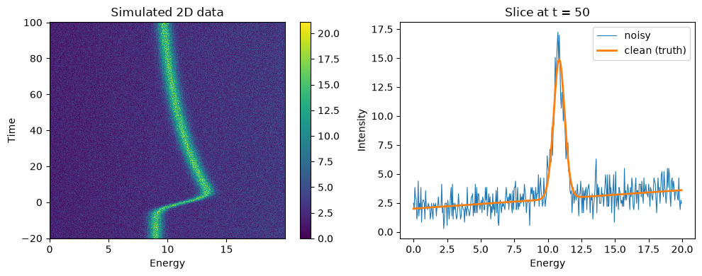
The data is a single 2D dataset: a GLP peak on a linear background. The GLP position shifts exponentially in time (convolved with a Gaussian instrument response function).

Ground truth model

• LinBack (linear background) + GLP peak — see models_energy_truth.yaml

• Time dependence on the peak position GLP_01_x0: expFun shift convolved with a gaussCONV IRF — see models_time_truth.yaml

Re-run this notebook to regenerate the data in place.

from pathlib import Path

import matplotlib.pyplot as plt
import numpy as np
import trspecfit

1. Define the Ground Truth Model

Build a 2D model on the same energy/time axes the example fits over. The *_truth.yaml files hold the ground truth parameters.

project = trspecfit.Project(path=Path.cwd(), config_file=None)

energy = np.arange(0, 20, 0.05)     # 400 points, 0.00 - 19.95
time = np.arange(-20, 100.25, 0.25)  # 481 points, -20.00 - 100.00

file = trspecfit.File(
    parent_project=project,
    energy=energy,
    time=time,
)

# Load the ground truth energy model and add the time dependence on the peak.
file.load_model(model_yaml='models_energy_truth.yaml', model_info='base')
file.add_time_dependence(
    target_model='base',
    target_parameter='GLP_01_x0',
    dynamics_yaml='models_time_truth.yaml',
    dynamics_model='MonoExpIRF',
)

file.describe_model()

Loading model to describe energy- (and time-)dependent data: base
Loading model to describe time-dependence of a model parameter: GLP_01_x0 of MonoExpIRF model
model name: base
function: LinBack from trspecfit.functions.energy
function: GLP from trspecfit.functions.energy
all lmfit.Parameters() [flattened and sorted alphabetically]:
Name                        Value      Min      Max   Stderr     Vary     Expr Brute_Step
GLP_01_A                       12     -inf      inf     None     True     None     None
GLP_01_F                        1     -inf      inf     None     True     None     None
GLP_01_m                     0.25     -inf      inf     None     True     None     None
GLP_01_x0                       9     -inf      inf     None     True     None     None
GLP_01_x0_expFun_01_A           5     -inf      inf     None     True     None     None
GLP_01_x0_expFun_01_t0          0     -inf      inf     None     True     None     None
GLP_01_x0_expFun_01_tau        50     -inf      inf     None     True     None     None
GLP_01_x0_gaussCONV_SD          3    1e-06       10     None     True     None     None
LinBack_b                       2     -inf      inf     None     True     None     None
LinBack_m                    0.08     -inf      inf     None     True     None     None
LinBack_xStart                  0     -inf      inf     None     True     None     None
LinBack_xStop                  20     -inf      inf     None     True     None     None

2. Simulate and Save

Photon-counting detection draws each pixel from a Poisson distribution, so the noise is signal-dependent (shot noise) — the realistic regime for counting detectors. Lower counts_per_delay ⇒ noisier data.

sim = trspecfit.Simulator(
    model=file.model_active,
    detection='photon_counting',
    counts_per_delay=5000,
    seed=42,
)
clean, noisy, noise = sim.simulate_2d()

# Save axes + noisy data (data is [time, energy], matching File's expectation).
data_fmt = '%.6e'
np.savetxt('energy.csv', energy, fmt=data_fmt)
np.savetxt('time.csv', time, fmt=data_fmt)
np.savetxt('data.csv', noisy, delimiter=',', fmt=data_fmt)

emask = (energy >= 5) & (energy <= 18)
snr = clean[:, emask].max() / np.std(noise[:, emask])
print(f'data.csv  |  shape {noisy.shape}  |  peak SNR ~ {snr:.1f}')

data.csv  |  shape (481, 400)  |  peak SNR ~ 14.6

3. Quick Visual Check

The 2D map shows the peak shifting in time; the 1D slice makes the noise level visible.

fig, axes = plt.subplots(1, 2, figsize=(10, 4))

im = axes[0].pcolormesh(energy, time, noisy, shading='auto')
axes[0].set_xlabel('Energy')
axes[0].set_ylabel('Time')
axes[0].set_title('Simulated 2D data')
plt.colorbar(im, ax=axes[0])

t_ind = np.abs(time - 50).argmin()
axes[1].plot(energy, noisy[t_ind], lw=0.8, label='noisy')
axes[1].plot(energy, clean[t_ind], lw=2.0, label='clean (truth)')
axes[1].set_xlabel('Energy')
axes[1].set_ylabel('Intensity')
axes[1].set_title(f'Slice at t = {time[t_ind]:.0f}')
axes[1].legend()

plt.tight_layout()
plt.show()

Ground Truth Parameters

Parameter	Value	Description
LinBack m	0.08	Background slope
LinBack b	2.0	Background intercept (at xStart)
LinBack xStart / xStop	0 / 20	Background clamp range
GLP A	12	Peak amplitude
GLP x0	9	Peak center (static part)
GLP F	1.0	Peak width
GLP m	0.25	Gaussian/Lorentzian mixing
gaussCONV SD	3	IRF width
expFun A	5	Peak-shift amplitude
expFun tau	50	Shift decay time constant
expFun t0	0	Time zero

Model files

The YAML files next to this notebook, as shipped with the example.

models_energy_truth.yaml

# ground truth energy model for data generation
# (same structure as the fit model in ../models_energy.yaml)

base:
    LinBack:
      m: [8E-2, True]
      b: [2.0, True]
      xStart: [0, True]
      xStop: [20, True]
    GLP:
      A: [12, True]
      x0: [9, True]
      F: [1.0, True]
      m: [0.25, True]

models_time_truth.yaml

# ground truth time model for data generation
# adds an exponential, IRF-convolved shift to the peak position

MonoExpIRF:
    gaussCONV:
        SD: [3, True, 1.0E-6, 10]
    expFun:
        A: [5, True]
        tau: [50, True]
        t0: [0, True]