Basic Fitting Workflow

This notebook demonstrates the standard fitting workflow for time- and energy-resolved spectroscopy data in five steps. The core is three models that build on each other:

1. Select the data: Load and inspect the data, then set the fit limits, i.e. energy/time region to fit.

2. Fit the baseline (base): Select the time slices making up the ground-state spectrum. Fit the well-determined line-shape parameters that are time-independent so the following fits are more robust and faster.

3. Slice-by-slice fitting (SbS): Fit each time slice independently, with the peak position being the only free fit parameter while the line shape is pinned to the baseline result. This reveals how the position moves in time without assuming a functional form.

4. Global 2D fitting (2D): Perform one global fit over the whole dataset, where the peak position follows a parametric law in time defined in models_time.yaml. This approach drastically reduces the overall number of free fit parameters compared to fitting a parametric law in time to the SbS fit results.

5. Inspect the results: compare the fitted values with the truth the data was generated from (data/models_energy_truth.yaml, data/models_time_truth.yaml).

from pathlib import Path

import numpy as np
import trspecfit

1. Load and Inspect Data

1.1 Load Data

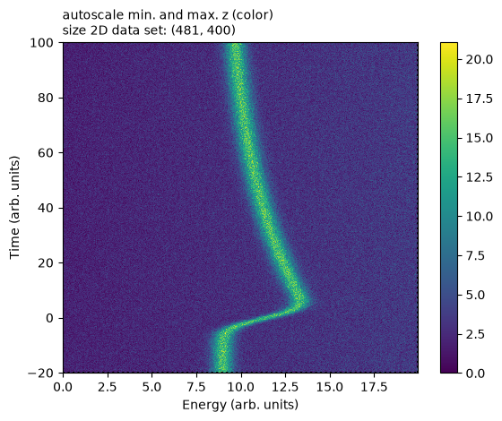
Load simulated time- and energy-resolved spectroscopy data from CSV files. The data is synthetic, generated by data/generate_data.ipynb which can be re-run to regenerate or change the data.

The 2D dataset is a stack of 1D energy spectra, one per time delay. The data array is [time, energy], i.e. rows are time, columns are energy.

# Create project
project = trspecfit.Project(path=Path.cwd())

# Directory containing data files
data_folder = 'data'

# Add file to project
file = trspecfit.File(
    parent_project=project,
    path=data_folder,
    data=np.loadtxt(project.path / data_folder / 'data.csv', delimiter=','),
    energy=np.loadtxt(project.path / data_folder / 'energy.csv'),
    time=np.loadtxt(project.path / data_folder / 'time.csv')
)

1.2 Inspect Data

A Gaussian–Lorentzian-product (GLP) peak sits on a linear background (LinBack). At t = 0 the peak position shifts to higher energy and relaxes back exponentially, blurred by a Gaussian instrument response (IRF).

# Visualize full dataset
file.describe()

File: data [path: data]

1.3 Define Fitting Region

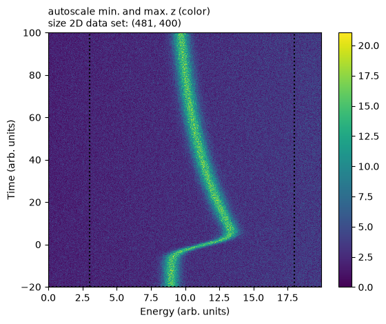
Set energy and time limits for the fits. They appear as black, dotted lines in the plot.

# Set fitting limits (absolute values)
file.set_fit_limits(
    energy_limits=[3, 18],  # Energy range
    time_limits=[-20, 100]  # Time range
)

2. Fit Baseline / Ground State Spectrum

2.1 Define Baseline Spectrum

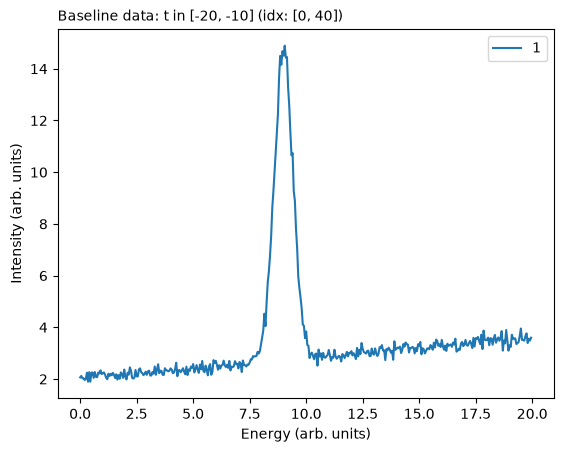
Extract the ground-state spectrum by averaging the pre-perturbation time slices. Make sure that the instrument response function is not bleeding into the baseline by lowering time_stop and re-fitting the baseline.

# Define baseline using absolute time values
file.define_baseline(
    time_start=-20,
    time_stop=-10,
    time_type='abs'  # Use absolute time values (or 'ind' for indices)
)

2.2 Fit Baseline Spectrum

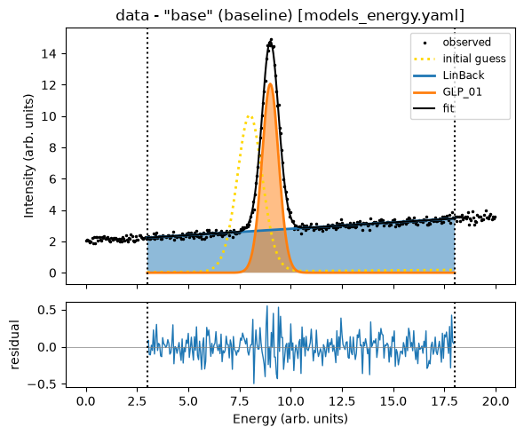
Fit the ground state spectrum leaving most fit parameters free to vary. The model is defined in models_energy.yaml. YAML model files are passed by name and resolved relative to the project directory passed to Project(...) in §1.1.

During time-dependent fits, the values of all fixed parameters (vary=False) will be set to the baseline fit result values.

The +/- values in the fit report below are lmfit’s defaults for a fit with no declared noise model; 12_uncertainty_mcmc declares the photon-counting noise this data carries and makes them right.

# Load baseline model
file.load_model(
    model_yaml='models_energy.yaml',
    model_info='base'
)

# Inspect model structure and parameters (detail=1 also plots the initial guess)
file.describe_model(model_info='base', detail=0)

Loading model to describe energy- (and time-)dependent data: base
model name: base
function: LinBack from trspecfit.functions.energy
function: GLP from trspecfit.functions.energy
all lmfit.Parameters() [flattened and sorted alphabetically]:
Name               Value      Min      Max   Stderr     Vary     Expr Brute_Step
GLP_01_A              10        5       15     None     True     None     None
GLP_01_F             1.5     0.75      2.5     None     True     None     None
GLP_01_m             0.3        0        1     None     True     None     None
GLP_01_x0              8        5       15     None     True     None     None
LinBack_b              0       -5        5     None     True     None     None
LinBack_m           0.01       -1        1     None     True     None     None
LinBack_xStart         0     -inf      inf     None    False     None     None
LinBack_xStop         20     -inf      inf     None    False     None     None

# Fit baseline model to data
# stages=1: single optimization
# stages=2: simplex pass, then leastsq refinement (see Tips)
file.fit_baseline(
    model_name='base',
    stages=2,
    try_ci=0  # skip confidence intervals: see 12_uncertainty_mcmc
)

Time initialize: 2.1696090698242188e-05 s

Results global minumum fit (method=Nelder): 
[[Variables]]
    LinBack_m:       0.23027807 +/- 0.01222682 (5.31%) (init = 0.01)
    LinBack_b:      -0.12080263 +/- 0.15189469 (125.74%) (init = 0)
    LinBack_xStart:  0 (fixed)
    LinBack_xStop:   20 (fixed)
    GLP_01_A:        10.2893013 +/- 0.27675792 (2.69%) (init = 10)
    GLP_01_x0:       8.98929513 +/- 0.01386768 (0.15%) (init = 8)
    GLP_01_F:        1.14778789 +/- 0.04533221 (3.95%) (init = 1.5)
    GLP_01_m:        0.99977913 +/- 0.00118739 (0.12%) (init = 0.3)
[[Correlations]] (unreported correlations are < 0.100)
    C(LinBack_m, LinBack_b) = -0.9063
    C(GLP_01_A, GLP_01_F)   = -0.5105
    C(LinBack_b, GLP_01_F)  = -0.3206
    C(LinBack_m, GLP_01_F)  = +0.1624
    C(LinBack_b, GLP_01_A)  = -0.1160
Time fit (global minimum): 0.11672425270080566 s

Results local optimization fit (method=leastsq): 
[[Variables]]
    LinBack_m:       0.08178437 +/- 0.00217330 (2.66%) (init = 0.01)
    LinBack_b:       1.98788819 +/- 0.02567974 (1.29%) (init = 0)
    LinBack_xStart:  0 (fixed)
    LinBack_xStop:   20 (fixed)
    GLP_01_A:        12.0596768 +/- 0.06241988 (0.52%) (init = 10)
    GLP_01_x0:       9.00139214 +/- 0.00205947 (0.02%) (init = 8)
    GLP_01_F:        0.99391770 +/- 0.00523400 (0.53%) (init = 1.5)
    GLP_01_m:        0.23296426 +/- 0.05601732 (24.05%) (init = 0.3)
[[Correlations]] (unreported correlations are < 0.100)
    C(LinBack_m, LinBack_b) = -0.9164
    C(GLP_01_A, GLP_01_m)   = +0.5302
    C(GLP_01_A, GLP_01_F)   = -0.4531
    C(LinBack_b, GLP_01_F)  = -0.1733
    C(LinBack_b, GLP_01_A)  = -0.1562
    C(LinBack_b, GLP_01_m)  = -0.1410
Time fit (local optimization): 0.00742030143737793 s
Time elapsed for baseline fit: 00.406(ss.ms)

Parameters

name	value	standard error	relative error	initial value	min	max	vary
LinBack_m	0.08178437	0.00217330	(2.66%)	0.01	-1.00000000	1.00000000	True
LinBack_b	1.98788819	0.02567974	(1.29%)	0.0	-5.00000000	5.00000000	True
LinBack_xStart	0.00000000	0.00000000		0.0	-inf	inf	False
LinBack_xStop	20.0000000	0.00000000	(0.00%)	20.0	-inf	inf	False
GLP_01_A	12.0596768	0.06241988	(0.52%)	10.0	5.00000000	15.0000000	True
GLP_01_x0	9.00139214	0.00205947	(0.02%)	8.0	5.00000000	15.0000000	True
GLP_01_F	0.99391770	0.00523400	(0.53%)	1.5	0.75000000	2.50000000	True
GLP_01_m	0.23296426	0.05601732	(24.05%)	0.3	0.00000000	1.00000000	True

3. Slice-by-Slice Fitting

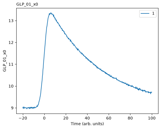
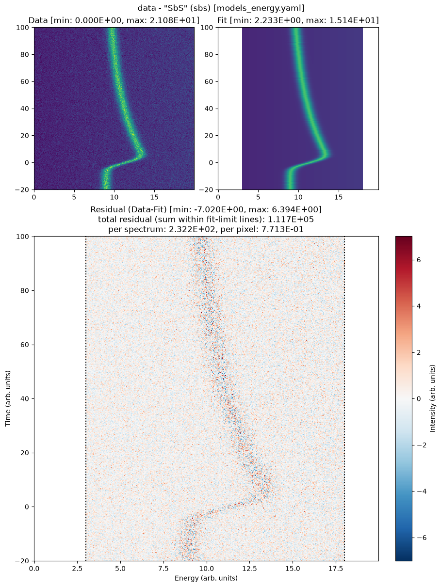
Fit each time slice independently to see how the parameters evolve over time, without assuming the form of that evolution. In this example, the peak position GLP_01_x0 is the only parameter free to vary as a function of time.

# Load Slice-by-Slice model
file.load_model(
    model_yaml='models_energy.yaml',
    model_info='SbS'
)

file.describe_model(model_info='SbS', detail=0)

Loading model to describe energy- (and time-)dependent data: SbS
model name: SbS
function: LinBack from trspecfit.functions.energy
function: GLP from trspecfit.functions.energy
all lmfit.Parameters() [flattened and sorted alphabetically]:
Name               Value      Min      Max   Stderr     Vary     Expr Brute_Step
GLP_01_A              12     -inf      inf     None    False     None     None
GLP_01_F             1.5     -inf      inf     None    False     None     None
GLP_01_m             0.3     -inf      inf     None    False     None     None
GLP_01_x0              8        5       15     None     True     None     None
LinBack_b              0     -inf      inf     None    False     None     None
LinBack_m           0.01     -inf      inf     None    False     None     None
LinBack_xStart         0     -inf      inf     None    False     None     None
LinBack_xStop         20     -inf      inf     None    False     None     None

# Perform Slice-by-Slice fit
file.fit_slice_by_slice(
    model_name='SbS',
    stages=1,
    try_ci=0  # Minimizer needs >=2 varying parameters to determine confidence intervals
)

SbS fit (15 workers): 100%|██████████| 481/481 [00:04<00:00, 102.85it/s]

Time elapsed for Slice-by-Slice fit: 06.724(ss.ms)

4. Global 2D Fitting

The slice-by-slice fit showed GLP_01_x0 jumping to higher energy at t = 0 and relaxing back toward its ground-state value: a shift-and-decay. So instead of leaving the position free in every slice, we model it with a single law in time. That law is an exponential shift-and-decay (expFun with positive A) convolved with a Gaussian instrument response (gaussCONV): the MonoExpIRF model in models_time.yaml.

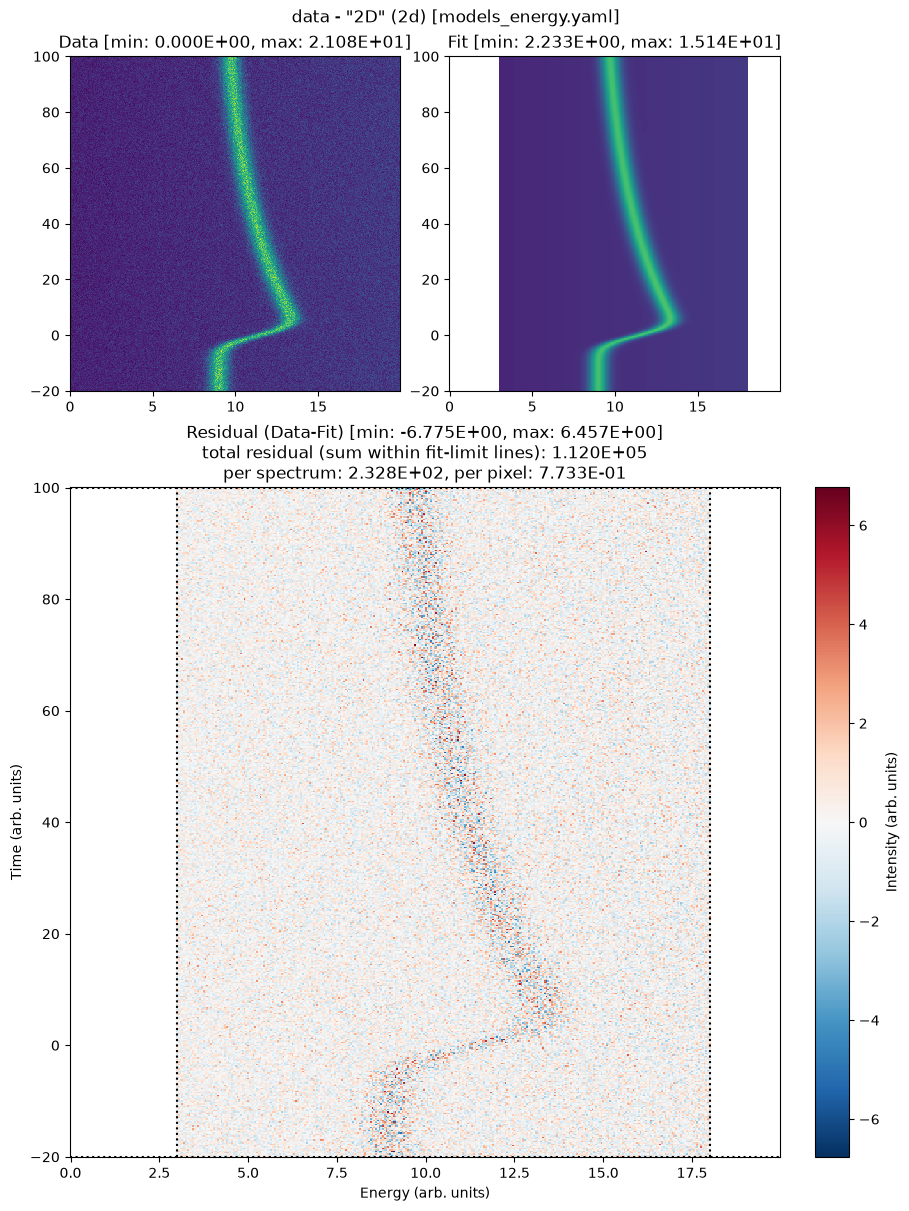
Why global? Fitting all time points together constrains the dynamics within the entire dataset, reducing overfitting and giving more robust, physically meaningful parameters than the independent per-slice fits. While one could fit the SbS results, i.e. GLP_01_x0(t) with the MonoExpIRF model, the overall number of free fit parameters in this approach would be hundreds more than in the global fit shown here.

# Load 2D model
file.load_model(
    model_yaml='models_energy.yaml',
    model_info='2D'
)

file.describe_model(model_info='2D', detail=0)

Loading model to describe energy- (and time-)dependent data: 2D
model name: 2D
function: LinBack from trspecfit.functions.energy
function: GLP from trspecfit.functions.energy
all lmfit.Parameters() [flattened and sorted alphabetically]:
Name               Value      Min      Max   Stderr     Vary     Expr Brute_Step
GLP_01_A              12     -inf      inf     None    False     None     None
GLP_01_F             1.5     -inf      inf     None    False     None     None
GLP_01_m             0.3     -inf      inf     None    False     None     None
GLP_01_x0              8        5       15     None     True     None     None
LinBack_b              0     -inf      inf     None    False     None     None
LinBack_m           0.01     -inf      inf     None    False     None     None
LinBack_xStart         0     -inf      inf     None    False     None     None
LinBack_xStop         20     -inf      inf     None    False     None     None

# Add time dependence to parameter
file.add_time_dependence(
    target_model='2D',
    target_parameter='GLP_01_x0',
    dynamics_yaml='models_time.yaml',
    dynamics_model='MonoExpIRF',
)

print("\n=== Model with Time Dependence ===")
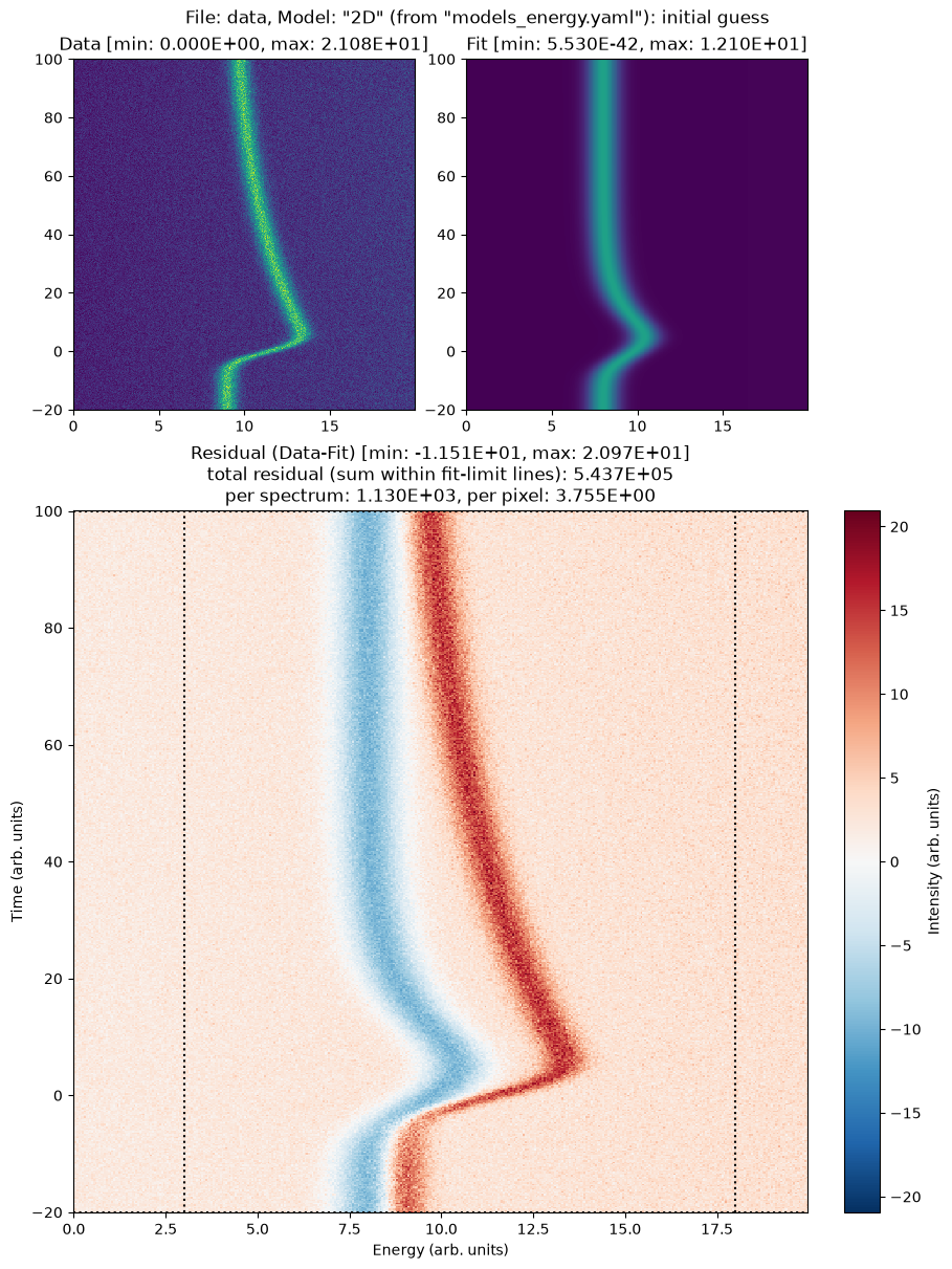
# detail=1 also plots the model at its initial guess
file.describe_model(model_info='2D', detail=1)

Loading model to describe time-dependence of a model parameter: GLP_01_x0 of MonoExpIRF model

=== Model with Time Dependence ===
model name: 2D
function: LinBack from trspecfit.functions.energy
function: GLP from trspecfit.functions.energy
all lmfit.Parameters() [flattened and sorted alphabetically]:
Name                        Value      Min      Max   Stderr     Vary     Expr Brute_Step
GLP_01_A                       12     -inf      inf     None    False     None     None
GLP_01_F                      1.5     -inf      inf     None    False     None     None
GLP_01_m                      0.3     -inf      inf     None    False     None     None
GLP_01_x0                       8        5       15     None     True     None     None
GLP_01_x0_expFun_01_A           5        0       15     None     True     None     None
GLP_01_x0_expFun_01_t0          0     -inf      inf     None    False     None     None
GLP_01_x0_expFun_01_tau        10        1      100     None     True     None     None
GLP_01_x0_gaussCONV_SD          5    1e-06       10     None     True     None     None
LinBack_b                       0     -inf      inf     None    False     None     None
LinBack_m                    0.01     -inf      inf     None    False     None     None
LinBack_xStart                  0     -inf      inf     None    False     None     None
LinBack_xStop                  20     -inf      inf     None    False     None     None

# Perform global 2D fit
file.fit_2d(
    model_name='2D',
    stages=2,
    try_ci=0  # skip confidence intervals: see 12_uncertainty_mcmc
)

Time initialize: 1.811981201171875e-05 s

Results global minumum fit (method=Nelder): 
[[Variables]]
    LinBack_m:                0.08178437 (fixed)
    LinBack_b:                1.987888 (fixed)
    LinBack_xStart:           0 (fixed)
    LinBack_xStop:            20 (fixed)
    GLP_01_A:                 12.05968 (fixed)
    GLP_01_x0:                8.90059080 +/- 0.00224013 (0.03%) (init = 9.001392)
    GLP_01_x0_gaussCONV_SD:   5.00000027 +/- 0.02706892 (0.54%) (init = 5)
    GLP_01_x0_expFun_01_A:    5.27602785 +/- 0.00422067 (0.08%) (init = 5)
    GLP_01_x0_expFun_01_tau:  49.9624606 +/- 0.05894668 (0.12%) (init = 10)
    GLP_01_x0_expFun_01_t0:   0 (fixed)
    GLP_01_F:                 0.9939177 (fixed)
    GLP_01_m:                 0.2329643 (fixed)
[[Correlations]] (unreported correlations are < 0.100)
    C(GLP_01_x0, GLP_01_x0_expFun_01_tau)             = -0.6617
    C(GLP_01_x0_gaussCONV_SD, GLP_01_x0_expFun_01_A)  = +0.6314
    C(GLP_01_x0, GLP_01_x0_expFun_01_A)               = -0.6013
    C(GLP_01_x0, GLP_01_x0_gaussCONV_SD)              = -0.5059
    C(GLP_01_x0_expFun_01_A, GLP_01_x0_expFun_01_tau) = -0.1066
Time fit (global minimum): 1.3580315113067627 s

Results local optimization fit (method=leastsq): 
[[Variables]]
    LinBack_m:                0.08178437 (fixed)
    LinBack_b:                1.987888 (fixed)
    LinBack_xStart:           0 (fixed)
    LinBack_xStop:            20 (fixed)
    GLP_01_A:                 12.05968 (fixed)
    GLP_01_x0:                9.00027992 +/- 0.00145395 (0.02%) (init = 9.001392)
    GLP_01_x0_gaussCONV_SD:   3.00427342 +/- 0.00652788 (0.22%) (init = 5)
    GLP_01_x0_expFun_01_A:    5.00053427 +/- 0.00262552 (0.05%) (init = 5)
    GLP_01_x0_expFun_01_tau:  49.9836079 +/- 0.04408199 (0.09%) (init = 10)
    GLP_01_x0_expFun_01_t0:   0 (fixed)
    GLP_01_F:                 0.9939177 (fixed)
    GLP_01_m:                 0.2329643 (fixed)
[[Correlations]] (unreported correlations are < 0.100)
    C(GLP_01_x0, GLP_01_x0_expFun_01_tau)             = -0.6526
    C(GLP_01_x0, GLP_01_x0_expFun_01_A)               = -0.5388
    C(GLP_01_x0_gaussCONV_SD, GLP_01_x0_expFun_01_A)  = +0.4300
    C(GLP_01_x0, GLP_01_x0_gaussCONV_SD)              = -0.2560
    C(GLP_01_x0_expFun_01_A, GLP_01_x0_expFun_01_tau) = -0.1494
Time fit (local optimization): 0.1859755516052246 s
Time elapsed for 2D model fit: 02.490(ss.ms)

Parameters

name	value	standard error	relative error	initial value	min	max	vary
LinBack_m	0.08178437	0.00000000	(0.00%)	0.0817843707272019	-inf	inf	False
LinBack_b	1.98788819	0.00000000	(0.00%)	1.987888192824693	-inf	inf	False
LinBack_xStart	0.00000000	0.00000000		0.0	-inf	inf	False
LinBack_xStop	20.0000000	0.00000000	(0.00%)	20.0	-inf	inf	False
GLP_01_A	12.0596768	0.00000000	(0.00%)	12.059676813726696	-inf	inf	False
GLP_01_x0	9.00027992	0.00145395	(0.02%)	9.001392138494767	5.00000000	15.0000000	True
GLP_01_x0_gaussCONV_SD	3.00427342	0.00652788	(0.22%)	5.0	1.0000e-06	10.0000000	True
GLP_01_x0_expFun_01_A	5.00053427	0.00262552	(0.05%)	5.0	0.00000000	15.0000000	True
GLP_01_x0_expFun_01_tau	49.9836079	0.04408199	(0.09%)	10.0	1.00000000	100.000000	True
GLP_01_x0_expFun_01_t0	0.00000000	0.00000000		0.0	-inf	inf	False
GLP_01_F	0.99391770	0.00000000	(0.00%)	0.9939177030931372	-inf	inf	False
GLP_01_m	0.23296426	0.00000000	(0.00%)	0.23296426434035067	-inf	inf	False

5. Inspect the Fit Results

file.get_parameters(fit_type=...) returns a pandas.DataFrame with one row per parameter for baseline / 2d or one row per time slice for sbs.
For more details on accessing fit results and metadata, see 10_model_comparison.

The data is synthetic, so the table below can be read against the truth in data/models_energy_truth.yaml and data/models_time_truth.yaml. The baseline fit recovers the peak shape (x0 = 9, A = 12, F = 1) and the linear background; the 2D fit recovers the dynamics (tau = 50, SD = 3, shift amplitude A = 5). The three fitted dynamics parameters land within one stderr of the truth. The line-shape parameters pinned from the baseline agree to within a few percent. The exception, GLP_01_m, is 0.3 σ from truth with a 24 % stderr: at this noise level, that is how well the line shape constrains m, which changes the curve little at small m and trades off against A and F.

# init_value is the seed each parameter started from: the YAML value, or the
# baseline result for the parameters the baseline pinned (those report stderr 0)
file.get_parameters(fit_type='2d')

	name	value	stderr	init_value	min	max	vary	expr
0	LinBack_m	0.081784	0.000000	0.081784	-inf	inf	False	None
1	LinBack_b	1.987888	0.000000	1.987888	-inf	inf	False	None
2	LinBack_xStart	0.000000	0.000000	0.000000	-inf	inf	False	None
3	LinBack_xStop	20.000000	0.000000	20.000000	-inf	inf	False	None
4	GLP_01_A	12.059677	0.000000	12.059677	-inf	inf	False	None
5	GLP_01_x0	9.000280	0.001454	9.001392	5.000000	15.0	True	None
6	GLP_01_x0_gaussCONV_SD	3.004273	0.006528	5.000000	0.000001	10.0	True	None
7	GLP_01_x0_expFun_01_A	5.000534	0.002626	5.000000	0.000000	15.0	True	None
8	GLP_01_x0_expFun_01_tau	49.983608	0.044082	10.000000	1.000000	100.0	True	None
9	GLP_01_x0_expFun_01_t0	0.000000	0.000000	0.000000	-inf	inf	False	None
10	GLP_01_F	0.993918	0.000000	0.993918	-inf	inf	False	None
11	GLP_01_m	0.232964	0.000000	0.232964	-inf	inf	False	None

Tips for Fitting

Fitting Strategy

• Always fit baseline first to establish good initial values

• Use Slice-by-Slice to identify which parameters are time-dependent

• Apply time-dependence only to parameters that clearly evolve

• Start with simple time-dependencies before complex ones

Fit Levels

• stages=1: Use a single optimization pass with e.g. least squares algorithm if your initial guess is close to the ground truth.

• stages=2: a derivative-free simplex pass (Nelder-Mead) first, which tolerates a rough initial guess and is less prone to settling in the nearest local minimum, then a least-squares refinement for precise values and uncertainties.

Common Fit Options

The fit_* methods expose stages directly and pass most other fit-control keywords through to trspecfit.fitlib.fit_wrapper.

Option	Applies to	Default	Use when
stages	baseline, SbS, 2D	1	1 runs fit_alg_1; 2 runs fit_alg_1 followed by fit_alg_2.
fit_alg_1	baseline, SbS, 2D	'Nelder'	Robust first pass. Use 'leastsq' for fast local fits when the initial guess is already close.
fit_alg_2	baseline, SbS, 2D	'leastsq'	Local refinement used only when stages=2.
try_ci	baseline, SbS, 2D	1	Set 0 for fast exploratory fits; set 1 for lmfit confidence intervals.
ci_sigmas	baseline, SbS, 2D	[1, 2, 3]	Confidence levels (in σ units) reported when try_ci=1.
mc_settings	baseline, SbS, 2D	off	Run MCMC uncertainty estimation; see 12_uncertainty_mcmc.
n_workers	SbS only	None	Control parallel Slice-by-Slice fitting; None auto-selects workers, 1 runs serially.
seed_source / seed_adapt	SbS only	'baseline' / 'argmax_shift'	Control how each independent time slice is initialized.

Next Steps

Uncertainty Estimation

• try_ci=1: Use lmfit.conf_interval for confidence intervals

• For robust MCMC-based uncertainty estimation, see 12_uncertainty_mcmc

Compare, Save & Export Fit Results

• For comparing two models on the same data, see 10_model_comparison

• To save, load, and export your fits — CSV/PNG for Origin / MATLAB, or round-trippable HDF5 archives, see 11_save_load_export

Explore More Complex Models

• For fitting with parameter expressions, see 02_dependent_parameters

• For fitting datasets with multiple sub-cycles, see 03_multi_cycle_dynamics

• For fit parameters that vary along an auxiliary axis, see 04_parameter_profiles

Model files

The YAML files next to this notebook, as shipped with the example.

models_energy.yaml

# Use these models to describe the energy-dependent data
# For available functions see: /src/trspecfit/functions/energy.py

# Ground state
# (most parameters vary here)
base:
    LinBack:
      m: [1E-2, True, -1, 1]
      b: [0, True, -5, 5]
      xStart: [0, False]
      xStop: [20, False]
    GLP:
      A: [10, True, 5, 15]
      x0: [8, True, 5, 15]
      F: [1.5, True, 0.75, 2.5]
      m: [0.3, True, 0, 1]

# Slice-by-Slice model fit
# (pinned parameters will be set to "base" Model fit result values)
SbS:
    LinBack:
      m: [1E-2, False]
      b: [0, False]
      xStart: [0, False]
      xStop: [20, False]
    GLP:
      A: [12, False]
      x0: [8, True, 5, 15]
      F: [1.5, False]
      m: [0.3, False]

# 2D model fit
# (pinned parameters will be set to "base" Model fit result values)
2D:
    LinBack:
      m: [1E-2, False]
      b: [0, False]
      xStart: [0, False]
      xStop: [20, False]
    GLP:
      A: [12, False]
      x0: [8, True, 5, 15]
      F: [1.5, False]
      m: [0.3, False]

models_time.yaml

# Use these models to add time-dependence to a parameter in a 2D model
# For available functions see: /src/trspecfit/functions/time.py

MonoExpIRF:
    gaussCONV:
        SD: [5, True, 1.0E-6, 10]
    expFun:
        A: [5, True, 0, 15]
        tau: [10, True, 1, 100]
        t0: [0, False]

project.yaml

# Project configuration for trspecfit basic_fitting example

# Display settings (general verbosity)
show_output: 1  # 0: silent/API mode, 1: interactive/notebook mode

# Axis labels
e_label: 'Energy (arb. units)' # x -> energy
t_label: 'Time (arb. units)' # y -> time
z_label: 'Intensity (arb. units)' # z -> intensity

# Plot settings
x_dir: 'def'  # def(ault) or rev(erse)
x_type: 'lin'  # lin or log
y_dir: 'def'  # def(ault) or rev(erse)
y_type: 'lin'  # lin or log
z_colormap: 'viridis' # colormap in 2D plots
z_type: 'lin'  # lin or log (2D plots)
dpi_plt: 100 # figure display dpi
dpi_save: 300 # figure save dpi
res_mult: 5 # residual multiplier in figures

The data were generated by data/generate_data.ipynb; its page shows the truth model files.