Parameter Profiles: Depth-Dependent Parameters#
This notebook shows how to let a model parameter vary along an auxiliary physical axis using a parameter profile. The example is time-resolved XPS of a semiconductor core level: XPS is surface-sensitive but not surface-exclusive, so the measured spectrum is a depth average — and two of the peak parameters depend on depth:
Amplitude (
GLP_01_A): signal from depth z is weighted byexp(-z / tau), wheretauis the inelastic mean free path (IMFP).Position (
GLP_01_x0): band bending shifts the binding energy linearly with depth,x0(z) = x0 + m·z.
The two ideas that drive everything here:
A profile makes one parameter a function of
aux_axis.file.add_par_profile(...)attaches a profile model (frommodels_profile.yaml) to a parameter; the component is then evaluated at everyaux_axispoint and the spectra are averaged — the model of a depth-integrated measurement. The profile’s parameters become regular fit parameters.Profile parameters can themselves be time-dependent.
add_time_dependencealso searches attached profiles, so the band bending gradientmcan carry the dynamics: photoexcitation at t = 0 collapses the band bending to flat-band condition and it recovers over ~100 ps. The depth profile then re-shapes at every time step (spectral diffusion) — the peak doesn’t just shift, its shape changes.
Workflow:
Select the data: load (including the depth axis), inspect, set fit limits.
Fit the baseline twice: a standard fit (effective, depth-averaged values) vs. a profile-aware fit (physical, surface values) — same data, different physics.
Slice-by-slice fitting (
SbS): track the band bending gradient through time, model-free.Profile-aware 2D fit (
2D): one global fit with the gradient’s time dependence.Inspect the results: compare to the known truth (
data/models_*_truth.yaml).
from pathlib import Path

import numpy as np
import trspecfit
1. Load and Inspect Data#
1.1 Load Data#
Load simulated time- and energy-resolved XPS data from CSV files. The data is synthetic, generated by data/generate_data.ipynb which can be re-run to regenerate or change the data.
The new ingredient compared to 01_basic_fitting is aux_axis — here the depth grid (nm) that profiles are evaluated on. It is not an axis of the data array (which stays [time, energy]); it is the integration grid for the depth average, set once on the File and inherited by every model loaded into it.
# Create project
project = trspecfit.Project(path=Path.cwd())

# Directory containing data files
data_folder = 'data'

# Add file to project (aux_axis: depth grid for the parameter profiles)
file = trspecfit.File(
    parent_project=project,
    path=data_folder,
    data=np.loadtxt(project.path / data_folder / 'data.csv', delimiter=','),
    energy=np.loadtxt(project.path / data_folder / 'energy.csv'),
    time=np.loadtxt(project.path / data_folder / 'time.csv'),
    aux_axis=np.loadtxt(project.path / data_folder / 'aux_axis.csv'),
)
1.2 Inspect Data#
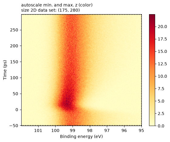
A single core-level peak (GLP) on a flat background (Offset). At t = 0 the peak jumps toward higher binding energy (the surface value), grows, and sharpens, then relaxes back over ~100 ps.
The growth and sharpening are the giveaway that this is more than a peak shift: at flat-band condition all depth layers line up at the same energy, so the depth average becomes taller and narrower. A time-dependent peak position alone (as in 01_basic_fitting) could never reproduce that — the shape of the spectrum changes.
# Visualize full dataset
file.describe()
File: data [path: data]
1.3 Define Fitting Region#
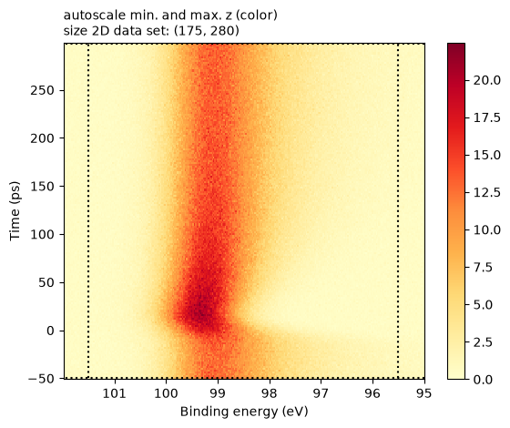
Set energy and time limits for the fits. They appear as black, dotted lines in the plot.
# Set fitting limits (absolute values)
file.set_fit_limits(
    energy_limits=[95.5, 101.5],  # Binding energy range (eV)
    time_limits=[-50, 298]  # Time range (ps)
)
2. Fit Baseline / Ground State Spectrum#
2.1 Define Baseline Spectrum#
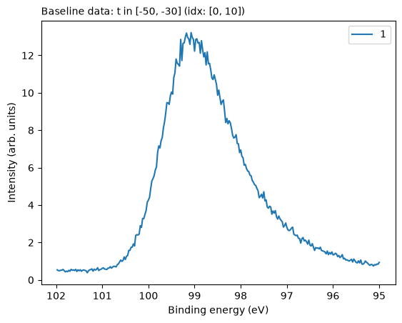
Extract the ground-state spectrum by averaging pre-excitation time slices. The Gaussian IRF (width ~10 ps) is non-causal — it bleeds the onset slightly before t = 0 — so stop the baseline at −30 ps, about 3 IRF widths.
# Define baseline using absolute time values
file.define_baseline(
    time_start=-50,
    time_stop=-30,
    time_type='abs'  # Use absolute time values (or 'ind' for indices)
)
2.2 Standard Fit — What a Depth-Blind Model Sees#
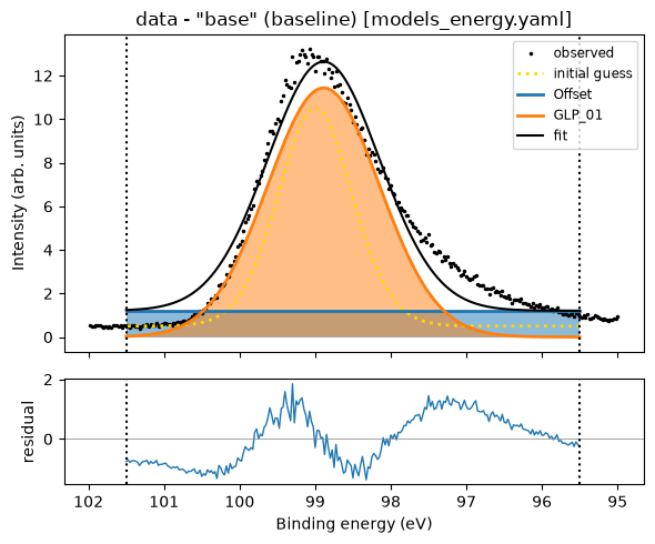
First fit the baseline with a plain GLP model (base in models_energy.yaml), no profiles. This converges happily, but every parameter is an effective, depth-averaged value. The amplitude bundles the IMFP weighting, the position sits below the surface binding energy (deeper layers sit at lower binding energy and pull the average down), and the width absorbs the band bending broadening. None of them is a physical property of the sample. Keep these numbers in mind for the comparison in section 5.
# Load standard baseline model (no profiles)
file.load_model(
    model_yaml='models_energy.yaml',
    model_info='base'
)

# Inspect model structure and parameters
file.describe_model(model_info='base', detail=0)
Loading model to describe energy- (and time-)dependent data: base
model name: base
function: Offset from trspecfit.functions.energy
function: GLP from trspecfit.functions.energy
all lmfit.Parameters() [flattened and sorted alphabetically]:
Name          Value      Min      Max   Stderr     Vary     Expr Brute_Step
GLP_01_A         10        1      100     None     True     None     None
GLP_01_F        1.2      0.5        5     None     True     None     None
GLP_01_m        0.3        0        1     None     True     None     None
GLP_01_x0        99       97      102     None     True     None     None
Offset_y0       0.5        0        3     None     True     None     None
# Fit standard baseline model to data
file.fit_baseline(
    model_name='base',
    stages=2,  # simplex pass, then leastsq refinement
    try_ci=0  # skip confidence intervals: see 12_uncertainty_mcmc
)
Time initialize: 2.3603439331054688e-05 s

Results global minumum fit (method=Nelder):
[[Variables]]
    Offset_y0:  1.19137478 +/- 0.11107788 (9.32%) (init = 0.5)
    GLP_01_A:   11.4709841 +/- 0.20189898 (1.76%) (init = 10)
    GLP_01_x0:  98.8886631 +/- 0.01116010 (0.01%) (init = 99)
    GLP_01_F:   1.79952576 +/- 0.04106297 (2.28%) (init = 1.2)
    GLP_01_m:   0.18800853 +/- 0.18887598 (100.46%) (init = 0.3)
[[Correlations]] (unreported correlations are < 0.100)
    C(Offset_y0, GLP_01_F)  = -0.7517
    C(GLP_01_A, GLP_01_m)   = +0.6471
    C(Offset_y0, GLP_01_A)  = -0.6012
    C(Offset_y0, GLP_01_m)  = -0.5323
    C(GLP_01_F, GLP_01_m)   = +0.5277
    C(GLP_01_A, GLP_01_F)   = +0.2430
    C(GLP_01_x0, GLP_01_F)  = -0.2002
    C(GLP_01_x0, GLP_01_m)  = +0.1330
    C(GLP_01_A, GLP_01_x0)  = +0.1222
    C(Offset_y0, GLP_01_x0) = +0.1066
Time fit (global minimum): 0.03537750244140625 s

Results local optimization fit (method=leastsq):
[[Variables]]
    Offset_y0:  1.20724550 +/- 0.11478521 (9.51%) (init = 0.5)
    GLP_01_A:   11.4345530 +/- 0.21345574 (1.87%) (init = 10)
    GLP_01_x0:  98.8881543 +/- 0.01047458 (0.01%) (init = 99)
    GLP_01_F:   1.79077464 +/- 0.06095140 (3.40%) (init = 1.2)
    GLP_01_m:   0.12750003 +/- 0.27479527 (215.53%) (init = 0.3)
[[Correlations]] (unreported correlations are < 0.100)
    C(GLP_01_F, GLP_01_m)  = +0.8454
    C(Offset_y0, GLP_01_F) = -0.7802
    C(GLP_01_A, GLP_01_m)  = +0.6959
    C(Offset_y0, GLP_01_A) = -0.6614
    C(Offset_y0, GLP_01_m) = -0.6074
    C(GLP_01_A, GLP_01_F)  = +0.5319
Time fit (local optimization): 0.00408172607421875 s
Time elapsed for baseline fit: 00.300(ss.ms)
| name | value | standard error | relative error | initial value | min | max | vary |
|---|---|---|---|---|---|---|---|
| Offset_y0 | 1.20724550 | 0.11478521 | (9.51%) | 0.5 | 0.00000000 | 3.00000000 | True |
| GLP_01_A | 11.4345530 | 0.21345574 | (1.87%) | 10.0 | 1.00000000 | 100.000000 | True |
| GLP_01_x0 | 98.8881543 | 0.01047458 | (0.01%) | 99.0 | 97.0000000 | 102.000000 | True |
| GLP_01_F | 1.79077464 | 0.06095140 | (3.40%) | 1.2 | 0.50000000 | 5.00000000 | True |
| GLP_01_m | 0.12750003 | 0.27479527 | (215.53%) | 0.3 | 0.00000000 | 1.00000000 | True |
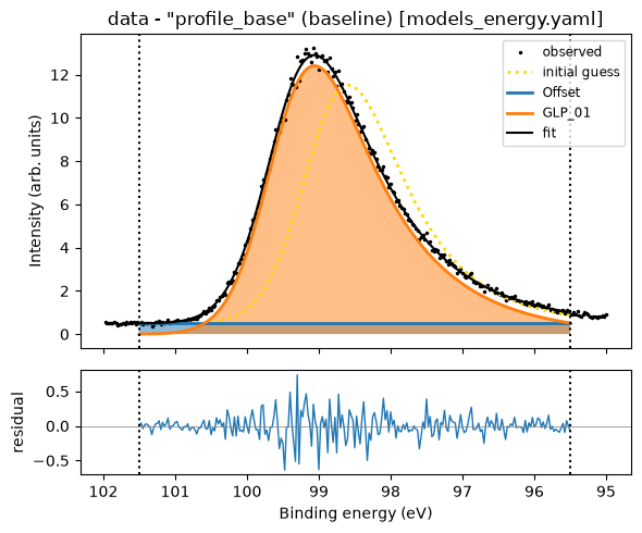
2.3 Profile-Aware Fit — Recovering the Physics#
Now load the same line shape with two depth profiles attached (profile_base). file.add_par_profile(...) works like add_time_dependence: it loads a profile model from a YAML file and attaches it to one parameter.
Profile model |
Target parameter |
Function |
Physical meaning |
|---|---|---|---|
|
|
|
surface sensitivity |
|
|
|
built-in electric field |
A profile adds to its base parameter at every depth point. Here A is fixed to 0, so the IMFP profile provides the full amplitude; x0 stays free as the surface binding energy, with the band bending shift m·z added on top. The profile’s parameters become regular fit parameters, named with the target parameter as prefix, e.g. GLP_01_x0_pLinear_01_m.
One parameter stays deliberately fixed: the IMFP tau. Rescaling (A, tau, m) → (c·A, tau/c, c·m) leaves the depth-averaged spectrum essentially unchanged, so fitting the IMFP together with the gradient is degenerate. Standard XPS practice applies: take the IMFP from tables (e.g. TPP-2M) for the material and kinetic energy, and fix it.
# Load the profile-aware baseline model (GLP A = 0, fixed)
file.load_model(
    model_yaml='models_energy.yaml',
    model_info='profile_base'
)

# Attach the IMFP amplitude profile
file.add_par_profile(
    target_model='profile_base',
    target_parameter='GLP_01_A',
    profile_yaml='models_profile.yaml',
    profile_model='IMFP'
)

# Attach the band bending position profile
file.add_par_profile(
    target_model='profile_base',
    target_parameter='GLP_01_x0',
    profile_yaml='models_profile.yaml',
    profile_model='BandBending'
)

file.describe_model(model_info='profile_base', detail=0)
Loading model to describe energy- (and time-)dependent data: profile_base
Loading profile model for parameter: GLP_01_A of IMFP model
Loading profile model for parameter: GLP_01_x0 of BandBending model
model name: profile_base
function: Offset from trspecfit.functions.energy
function: GLP from trspecfit.functions.energy
all lmfit.Parameters() [flattened and sorted alphabetically]:
Name                          Value      Min      Max   Stderr     Vary     Expr Brute_Step
GLP_01_A                          0     -inf      inf     None    False     None     None
GLP_01_A_pExpDecay_01_A          80        1     1000     None     True     None     None
GLP_01_A_pExpDecay_01_tau         2     -inf      inf     None    False     None     None
GLP_01_F                        1.2      0.5        5     None     True     None     None
GLP_01_m                        0.3        0        1     None     True     None     None
GLP_01_x0                        99       97      102     None     True     None     None
GLP_01_x0_pLinear_01_b            0     -inf      inf     None    False     None     None
GLP_01_x0_pLinear_01_m         -0.4       -2        0     None     True     None     None
Offset_y0                       0.5        0        3     None     True     None     None
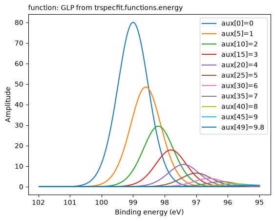
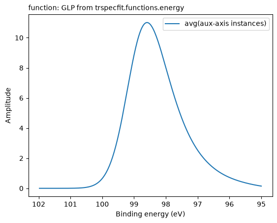
# Visualize the profiled GLP component: one trace per depth point (deeper
# layers are weaker from the IMFP weight and shifted by the band bending),
# then the depth-averaged spectrum that is actually compared to the data.
c_GLP = file.model_active.components[1]
c_GLP.plot(plot_every=5)  # plot every 5th depth trace
c_GLP.plot(plot_traces=False)  # depth-averaged spectrum
# Fit profile-aware baseline model to data
file.fit_baseline(
    model_name='profile_base',
    stages=2,
    try_ci=0  # skip confidence intervals: see 12_uncertainty_mcmc
)
Time initialize: 1.5974044799804688e-05 s

Results global minumum fit (method=Nelder):
[[Variables]]
    Offset_y0:                  0.49509553 +/- 0.02703661 (5.46%) (init = 0.5)
    GLP_01_A:                   0 (fixed)
    GLP_01_A_pExpDecay_01_A:    100.736434 +/- 1.01195422 (1.00%) (init = 80)
    GLP_01_A_pExpDecay_01_tau:  2 (fixed)
    GLP_01_x0:                  99.5076997 +/- 0.00364493 (0.00%) (init = 99)
    GLP_01_x0_pLinear_01_m:    -0.50115206 +/- 0.00498435 (0.99%) (init = -0.4)
    GLP_01_x0_pLinear_01_b:     0 (fixed)
    GLP_01_F:                   1.18603902 +/- 0.01243745 (1.05%) (init = 1.2)
    GLP_01_m:                   0.33567472 +/- 0.07793735 (23.22%) (init = 0.3)
[[Correlations]] (unreported correlations are < 0.100)
    C(GLP_01_A_pExpDecay_01_A, GLP_01_F)               = -0.8304
    C(GLP_01_x0, GLP_01_x0_pLinear_01_m)               = -0.8233
    C(GLP_01_F, GLP_01_m)                              = -0.7329
    C(GLP_01_A_pExpDecay_01_A, GLP_01_x0_pLinear_01_m) = -0.5737
    C(GLP_01_A_pExpDecay_01_A, GLP_01_m)               = +0.5737
    C(Offset_y0, GLP_01_A_pExpDecay_01_A)              = -0.5443
    C(GLP_01_A_pExpDecay_01_A, GLP_01_x0)              = +0.4724
    C(Offset_y0, GLP_01_x0_pLinear_01_m)               = +0.4668
    C(Offset_y0, GLP_01_x0)                            = -0.3971
    C(Offset_y0, GLP_01_m)                             = -0.3957
    C(GLP_01_x0_pLinear_01_m, GLP_01_m)                = +0.1653
    C(Offset_y0, GLP_01_F)                             = +0.1510
    C(GLP_01_x0_pLinear_01_m, GLP_01_F)                = +0.1361
    C(GLP_01_x0, GLP_01_m)                             = -0.1341
    C(GLP_01_x0, GLP_01_F)                             = -0.1074
Time fit (global minimum): 0.25925350189208984 s

Results local optimization fit (method=leastsq):
[[Variables]]
    Offset_y0:                  0.49416357 +/- 0.02713813 (5.49%) (init = 0.5)
    GLP_01_A:                   0 (fixed)
    GLP_01_A_pExpDecay_01_A:    100.788593 +/- 1.02054150 (1.01%) (init = 80)
    GLP_01_A_pExpDecay_01_tau:  2 (fixed)
    GLP_01_x0:                  99.5076488 +/- 0.00363757 (0.00%) (init = 99)
    GLP_01_x0_pLinear_01_m:    -0.50106483 +/- 0.00497114 (0.99%) (init = -0.4)
    GLP_01_x0_pLinear_01_b:     0 (fixed)
    GLP_01_F:                   1.18517880 +/- 0.01268828 (1.07%) (init = 1.2)
    GLP_01_m:                   0.34285186 +/- 0.07658229 (22.34%) (init = 0.3)
[[Correlations]] (unreported correlations are < 0.100)
    C(GLP_01_A_pExpDecay_01_A, GLP_01_F)               = -0.8331
    C(GLP_01_x0, GLP_01_x0_pLinear_01_m)               = -0.8225
    C(GLP_01_F, GLP_01_m)                              = -0.7442
    C(GLP_01_A_pExpDecay_01_A, GLP_01_x0_pLinear_01_m) = -0.5821
    C(GLP_01_A_pExpDecay_01_A, GLP_01_m)               = +0.5807
    C(Offset_y0, GLP_01_A_pExpDecay_01_A)              = -0.5482
    C(GLP_01_A_pExpDecay_01_A, GLP_01_x0)              = +0.4840
    C(Offset_y0, GLP_01_x0_pLinear_01_m)               = +0.4709
    C(Offset_y0, GLP_01_m)                             = -0.4049
    C(Offset_y0, GLP_01_x0)                            = -0.4028
    C(Offset_y0, GLP_01_F)                             = +0.1660
    C(GLP_01_x0_pLinear_01_m, GLP_01_F)                = +0.1466
    C(GLP_01_x0_pLinear_01_m, GLP_01_m)                = +0.1463
    C(GLP_01_x0, GLP_01_F)                             = -0.1222
    C(GLP_01_x0, GLP_01_m)                             = -0.1114
Time fit (local optimization): 0.009808778762817383 s
Time elapsed for baseline fit: 00.529(ss.ms)
| name | value | standard error | relative error | initial value | min | max | vary |
|---|---|---|---|---|---|---|---|
| Offset_y0 | 0.49416357 | 0.02713813 | (5.49%) | 0.5 | 0.00000000 | 3.00000000 | True |
| GLP_01_A | 0.00000000 | 0.00000000 | 0.0 | -inf | inf | False | |
| GLP_01_A_pExpDecay_01_A | 100.788593 | 1.02054150 | (1.01%) | 80.0 | 1.00000000 | 1000.00000 | True |
| GLP_01_A_pExpDecay_01_tau | 2.00000000 | 0.00000000 | (0.00%) | 2.0 | -inf | inf | False |
| GLP_01_x0 | 99.5076488 | 0.00363757 | (0.00%) | 99.0 | 97.0000000 | 102.000000 | True |
| GLP_01_x0_pLinear_01_m | -0.50106483 | 0.00497114 | (0.99%) | -0.4 | -2.00000000 | 0.00000000 | True |
| GLP_01_x0_pLinear_01_b | 0.00000000 | 0.00000000 | 0.0 | -inf | inf | False | |
| GLP_01_F | 1.18517880 | 0.01268828 | (1.07%) | 1.2 | 0.50000000 | 5.00000000 | True |
| GLP_01_m | 0.34285186 | 0.07658229 | (22.34%) | 0.3 | 0.00000000 | 1.00000000 | True |
3. Slice-by-Slice Fitting#
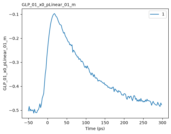
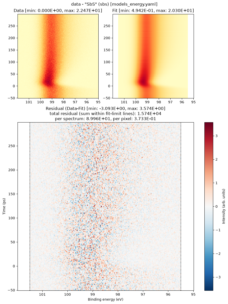
Fit each time slice independently with exactly one free parameter: the band bending gradient GLP_01_x0_pLinear_01_m. The SbS energy model pins all line-shape parameters, and the IMFPfixed profile variant pins the IMFP amplitude — all pinned values are seeded from the profile_base fit results.
The result is the gradient-vs-time trace without assuming any functional form — look for the jump from −0.5 to ≈ 0 eV/nm at t = 0 (flat-band condition) and the exponential recovery, with the onset smoothed by the IRF. That trace is what motivates the dynamics model in section 4.
# Load Slice-by-Slice model and attach the profiles
file.load_model(
    model_yaml='models_energy.yaml',
    model_info='SbS'
)

file.add_par_profile(
    target_model='SbS',
    target_parameter='GLP_01_A',
    profile_yaml='models_profile.yaml',
    profile_model='IMFPfixed'  # pinned variant: amplitude profile stays fixed
)
file.add_par_profile(
    target_model='SbS',
    target_parameter='GLP_01_x0',
    profile_yaml='models_profile.yaml',
    profile_model='BandBending'  # gradient m is the one free parameter
)

file.describe_model(model_info='SbS', detail=0)
Loading model to describe energy- (and time-)dependent data: SbS
Loading profile model for parameter: GLP_01_A of IMFPfixed model
Loading profile model for parameter: GLP_01_x0 of BandBending model
model name: SbS
function: Offset from trspecfit.functions.energy
function: GLP from trspecfit.functions.energy
all lmfit.Parameters() [flattened and sorted alphabetically]:
Name                          Value      Min      Max   Stderr     Vary     Expr Brute_Step
GLP_01_A                          0     -inf      inf     None    False     None     None
GLP_01_A_pExpDecay_01_A          80     -inf      inf     None    False     None     None
GLP_01_A_pExpDecay_01_tau         2     -inf      inf     None    False     None     None
GLP_01_F                        1.2     -inf      inf     None    False     None     None
GLP_01_m                        0.3     -inf      inf     None    False     None     None
GLP_01_x0                        99     -inf      inf     None    False     None     None
GLP_01_x0_pLinear_01_b            0     -inf      inf     None    False     None     None
GLP_01_x0_pLinear_01_m         -0.4       -2        0     None     True     None     None
Offset_y0                       0.5     -inf      inf     None    False     None     None
# Perform Slice-by-Slice fit
file.fit_slice_by_slice(
    model_name='SbS',
    stages=1,  # one optimizer pass per slice, seeded from the profile_base fit
    try_ci=0  # Minimizer needs >=2 varying parameters to determine confidence intervals
)
SbS fit (15 workers): 100%|██████████| 175/175 [00:03<00:00, 46.64it/s]
Time elapsed for Slice-by-Slice fit: 05.595(ss.ms)
4. Profile-Aware Global 2D Fitting#
The missing piece is the gradient’s time dependence:
file.add_time_dependence(..., target_parameter='GLP_01_x0_pLinear_01_m', ...)
The target is a profile parameter.
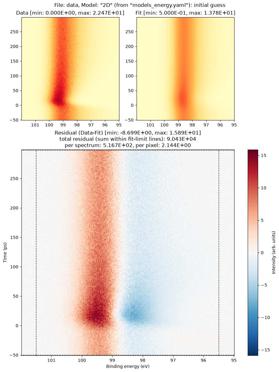
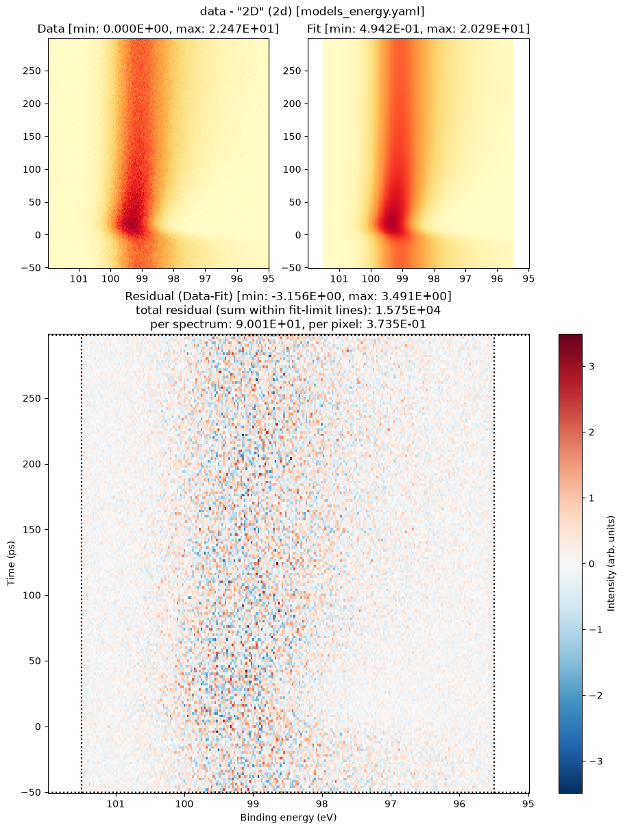
add_time_dependencesearches the energy model first and then every attached profile — so attach the profile before adding the time dependence. The model’sdimis promoted to 2 automatically.Spectral diffusion. At every time step the depth profile is re-evaluated with the current gradient, so the whole depth-averaged line shape responds — reproducing the grow-and-sharpen transient from section 1.2.
What varies globally: the surface position
x0, the equilibrium gradientm, and the three dynamics parameters ofBandBendingRecovery(models_time.yaml): IRF widthSD, collapse amplitudeA, recovery timetau. Line shape and IMFP amplitude stay pinned to theprofile_baseresults.
# Load 2D model and attach the profiles
file.load_model(
    model_yaml='models_energy.yaml',
    model_info='2D'
)

file.add_par_profile(
    target_model='2D',
    target_parameter='GLP_01_A',
    profile_yaml='models_profile.yaml',
    profile_model='IMFPfixed'  # pinned variant: amplitude profile stays fixed
)
file.add_par_profile(
    target_model='2D',
    target_parameter='GLP_01_x0',
    profile_yaml='models_profile.yaml',
    profile_model='BandBending'
)

# Add time dependence to the band bending gradient (a profile parameter)
file.add_time_dependence(
    target_model='2D',
    target_parameter='GLP_01_x0_pLinear_01_m',
    dynamics_yaml='models_time.yaml',
    dynamics_model='BandBendingRecovery'
)

print("\n=== Model with Time-Dependent Profile Parameter ===")
file.describe_model(model_info='2D', detail=1)
Loading model to describe energy- (and time-)dependent data: 2D
Loading profile model for parameter: GLP_01_A of IMFPfixed model
Loading profile model for parameter: GLP_01_x0 of BandBending model
Loading model to describe time-dependence of a model parameter: GLP_01_x0_pLinear_01_m of BandBendingRecovery model

=== Model with Time-Dependent Profile Parameter ===
model name: 2D
function: Offset from trspecfit.functions.energy
function: GLP from trspecfit.functions.energy
all lmfit.Parameters() [flattened and sorted alphabetically]:
Name                                     Value      Min      Max   Stderr     Vary     Expr Brute_Step
GLP_01_A                                     0     -inf      inf     None    False     None     None
GLP_01_A_pExpDecay_01_A                     80     -inf      inf     None    False     None     None
GLP_01_A_pExpDecay_01_tau                    2     -inf      inf     None    False     None     None
GLP_01_F                                   1.2     -inf      inf     None    False     None     None
GLP_01_m                                   0.3     -inf      inf     None    False     None     None
GLP_01_x0                                   99       97      102     None     True     None     None
GLP_01_x0_pLinear_01_b                       0     -inf      inf     None    False     None     None
GLP_01_x0_pLinear_01_m                    -0.4       -2        0     None     True     None     None
GLP_01_x0_pLinear_01_m_expFun_01_A         0.3        0        1     None     True     None     None
GLP_01_x0_pLinear_01_m_expFun_01_t0          0     -inf      inf     None    False     None     None
GLP_01_x0_pLinear_01_m_expFun_01_tau        50        5      500     None     True     None     None
GLP_01_x0_pLinear_01_m_gaussCONV_SD         20        1       50     None     True     None     None
Offset_y0                                  0.5     -inf      inf     None    False     None     None
# Perform global 2D fit
file.fit_2d(
    model_name='2D',
    stages=2,
    try_ci=0  # skip confidence intervals: see 12_uncertainty_mcmc
)
Time initialize: 9.059906005859375e-06 s

Results global minumum fit (method=Nelder):
[[Variables]]
    Offset_y0:                             0.4941636 (fixed)
    GLP_01_A:                              0 (fixed)
    GLP_01_A_pExpDecay_01_A:               100.7886 (fixed)
    GLP_01_A_pExpDecay_01_tau:             2 (fixed)
    GLP_01_x0:                             99.5014449 +/- 5.2662e-04 (0.00%) (init = 99.50765)
    GLP_01_x0_pLinear_01_m:               -0.49858495 +/- 8.6572e-04 (0.17%) (init = -0.5010648)
    GLP_01_x0_pLinear_01_b:                0 (fixed)
    GLP_01_x0_pLinear_01_m_gaussCONV_SD:   10.1037007 +/- 0.08305696 (0.82%) (init = 20)
    GLP_01_x0_pLinear_01_m_expFun_01_A:    0.49757377 +/- 0.00122951 (0.25%) (init = 0.3)
    GLP_01_x0_pLinear_01_m_expFun_01_tau:  98.9802556 +/- 0.53733866 (0.54%) (init = 50)
    GLP_01_x0_pLinear_01_m_expFun_01_t0:   0 (fixed)
    GLP_01_F:                              1.185179 (fixed)
    GLP_01_m:                              0.3428519 (fixed)
[[Correlations]] (unreported correlations are < 0.100)
    C(GLP_01_x0_pLinear_01_m, GLP_01_x0_pLinear_01_m_expFun_01_tau)              = -0.6923
    C(GLP_01_x0_pLinear_01_m_gaussCONV_SD, GLP_01_x0_pLinear_01_m_expFun_01_A)   = +0.5469
    C(GLP_01_x0_pLinear_01_m, GLP_01_x0_pLinear_01_m_expFun_01_A)                = -0.4749
    C(GLP_01_x0_pLinear_01_m_gaussCONV_SD, GLP_01_x0_pLinear_01_m_expFun_01_tau) = -0.3811
    C(GLP_01_x0, GLP_01_x0_pLinear_01_m)                               = -0.2921
    C(GLP_01_x0_pLinear_01_m_expFun_01_A, GLP_01_x0_pLinear_01_m_expFun_01_tau)  = -0.1256
Time fit (global minimum): 21.700589418411255 s

Results local optimization fit (method=leastsq):
[[Variables]]
    Offset_y0:                             0.4941636 (fixed)
    GLP_01_A:                              0 (fixed)
    GLP_01_A_pExpDecay_01_A:               100.7886 (fixed)
    GLP_01_A_pExpDecay_01_tau:             2 (fixed)
    GLP_01_x0:                             99.5014506 +/- 5.2566e-04 (0.00%) (init = 99.50765)
    GLP_01_x0_pLinear_01_m:               -0.49857935 +/- 8.6707e-04 (0.17%) (init = -0.5010648)
    GLP_01_x0_pLinear_01_b:                0 (fixed)
    GLP_01_x0_pLinear_01_m_gaussCONV_SD:   10.1035516 +/- 0.08379239 (0.83%) (init = 20)
    GLP_01_x0_pLinear_01_m_expFun_01_A:    0.49756443 +/- 0.00123020 (0.25%) (init = 0.3)
    GLP_01_x0_pLinear_01_m_expFun_01_tau:  98.9792531 +/- 0.53819081 (0.54%) (init = 50)
    GLP_01_x0_pLinear_01_m_expFun_01_t0:   0 (fixed)
    GLP_01_F:                              1.185179 (fixed)
    GLP_01_m:                              0.3428519 (fixed)
[[Correlations]] (unreported correlations are < 0.100)
    C(GLP_01_x0_pLinear_01_m, GLP_01_x0_pLinear_01_m_expFun_01_tau)              = -0.6923
    C(GLP_01_x0_pLinear_01_m_gaussCONV_SD, GLP_01_x0_pLinear_01_m_expFun_01_A)   = +0.5462
    C(GLP_01_x0_pLinear_01_m, GLP_01_x0_pLinear_01_m_expFun_01_A)                = -0.4743
    C(GLP_01_x0_pLinear_01_m_gaussCONV_SD, GLP_01_x0_pLinear_01_m_expFun_01_tau) = -0.3817
    C(GLP_01_x0, GLP_01_x0_pLinear_01_m)                               = -0.2919
    C(GLP_01_x0_pLinear_01_m_expFun_01_A, GLP_01_x0_pLinear_01_m_expFun_01_tau)  = -0.1266
Time fit (local optimization): 0.4961225986480713 s
Time elapsed for 2D model fit: 22.926(ss.ms)
| name | value | standard error | relative error | initial value | min | max | vary |
|---|---|---|---|---|---|---|---|
| Offset_y0 | 0.49416357 | 0.00000000 | (0.00%) | 0.4941635694565138 | -inf | inf | False |
| GLP_01_A | 0.00000000 | 0.00000000 | 0.0 | -inf | inf | False | |
| GLP_01_A_pExpDecay_01_A | 100.788593 | 0.00000000 | (0.00%) | 100.78859266824419 | -inf | inf | False |
| GLP_01_A_pExpDecay_01_tau | 2.00000000 | 0.00000000 | (0.00%) | 2.0 | -inf | inf | False |
| GLP_01_x0 | 99.5014506 | 5.2566e-04 | (0.00%) | 99.50764878915689 | 97.0000000 | 102.000000 | True |
| GLP_01_x0_pLinear_01_m | -0.49857935 | 8.6707e-04 | (0.17%) | -0.5010648261135402 | -2.00000000 | 0.00000000 | True |
| GLP_01_x0_pLinear_01_b | 0.00000000 | 0.00000000 | 0.0 | -inf | inf | False | |
| GLP_01_x0_pLinear_01_m_gaussCONV_SD | 10.1035516 | 0.08379239 | (0.83%) | 20.0 | 1.00000000 | 50.0000000 | True |
| GLP_01_x0_pLinear_01_m_expFun_01_A | 0.49756443 | 0.00123020 | (0.25%) | 0.3 | 0.00000000 | 1.00000000 | True |
| GLP_01_x0_pLinear_01_m_expFun_01_tau | 98.9792531 | 0.53819081 | (0.54%) | 50.0 | 5.00000000 | 500.000000 | True |
| GLP_01_x0_pLinear_01_m_expFun_01_t0 | 0.00000000 | 0.00000000 | 0.0 | -inf | inf | False | |
| GLP_01_F | 1.18517880 | 0.00000000 | (0.00%) | 1.1851787986179445 | -inf | inf | False |
| GLP_01_m | 0.34285186 | 0.00000000 | (0.00%) | 0.3428518631251885 | -inf | inf | False |
5. Inspect the Fit Results#
file.get_parameters(fit_type='2d') returns a pandas.DataFrame with one row per parameter. The names chain target parameter → profile → dynamics: GLP_01_x0_pLinear_01_m_expFun_01_tau reads as “the tau of the expFun dynamics on the pLinear gradient of the GLP position”.
Because the data is synthetic, the results can be compared to the known truth (data/models_*_truth.yaml):
The standard baseline fit (section 2.2) returned effective values — amplitude ≈ 11, position ≈ 98.9 eV, width ≈ 1.8 eV — none of which is a physical property of the sample (truth: surface weight 100, surface binding energy 99.5 eV, FWHM 1.2 eV).
The profile-aware fits recover the physics: surface weight
pExpDecay_01_A ≈ 100, surface binding energyx0 ≈ 99.5 eV, equilibrium gradientpLinear_01_m ≈ −0.5 eV/nm, IRF widthSD ≈ 10 ps, collapse amplitudeexpFun_01_A ≈ +0.5 eV/nm, and recovery timetau ≈ 100 ps.Note the collapse amplitude: it cancels the equilibrium gradient at t = 0 — the fit has measured that the photovoltage drives the bands all the way to flat-band condition.
file.get_parameters(fit_type='2d')
| name | value | stderr | init_value | min | max | vary | expr | |
|---|---|---|---|---|---|---|---|---|
| 0 | Offset_y0 | 0.494164 | 0.000000 | 0.494164 | -inf | inf | False | None |
| 1 | GLP_01_A | 0.000000 | 0.000000 | 0.000000 | -inf | inf | False | None |
| 2 | GLP_01_A_pExpDecay_01_A | 100.788593 | 0.000000 | 100.788593 | -inf | inf | False | None |
| 3 | GLP_01_A_pExpDecay_01_tau | 2.000000 | 0.000000 | 2.000000 | -inf | inf | False | None |
| 4 | GLP_01_x0 | 99.501451 | 0.000526 | 99.507649 | 97.0 | 102.0 | True | None |
| 5 | GLP_01_x0_pLinear_01_m | -0.498579 | 0.000867 | -0.501065 | -2.0 | 0.0 | True | None |
| 6 | GLP_01_x0_pLinear_01_b | 0.000000 | 0.000000 | 0.000000 | -inf | inf | False | None |
| 7 | GLP_01_x0_pLinear_01_m_gaussCONV_SD | 10.103552 | 0.083792 | 20.000000 | 1.0 | 50.0 | True | None |
| 8 | GLP_01_x0_pLinear_01_m_expFun_01_A | 0.497564 | 0.001230 | 0.300000 | 0.0 | 1.0 | True | None |
| 9 | GLP_01_x0_pLinear_01_m_expFun_01_tau | 98.979253 | 0.538191 | 50.000000 | 5.0 | 500.0 | True | None |
| 10 | GLP_01_x0_pLinear_01_m_expFun_01_t0 | 0.000000 | 0.000000 | 0.000000 | -inf | inf | False | None |
| 11 | GLP_01_F | 1.185179 | 0.000000 | 1.185179 | -inf | inf | False | None |
| 12 | GLP_01_m | 0.342852 | 0.000000 | 0.342852 | -inf | inf | False | None |
Tips for Profile Fitting#
Profile basics
Set
aux_axisonce onFile(...); every loaded model inherits it.A profile adds to its base parameter at each aux point. Fix the base parameter to 0 when the profile should provide the entire value (amplitude); keep it free when the profile is a relative shift (position).
Vary flags of profile parameters live in the profile YAML like everywhere else — pinned variants (e.g.
IMFPfixed) are just additional entries inmodels_profile.yaml, and pinned parameters inherit the baseline fit values.
Identifiability
Depth profiles extracted from a single spectrum are strongly correlated (here: an exact scaling degeneracy between IMFP and gradient). Fix what is known independently — the IMFP from tables — and check the reported correlations before trusting profile parameters.
Time-dependent profile parameters
Attach the profile first, then call
add_time_dependenceon the profile parameter ({target_par}_{component}_{par}name); the model is promoted to 2D automatically.
Available profile functions (src/trspecfit/functions/profile.py)
pExpDecay(x, A, tau)— IMFP weighting, Beer-Lambert absorptionpLinear(x, m, b)— band bending, linear gradientspGauss(x, A, x0, SD)— fluence averaging, inhomogeneous broadening
Next Steps#
Is the profile model justified by the data? Fit both variants and compare:
10_model_comparisonUncertainty estimation (MCMC):
12_uncertainty_mcmcSave, load, and export fits:
11_save_load_export
Model files#
The YAML files next to this notebook, as shipped with the example.
models_energy.yaml#
# Energy models for the parameter-profiles example
# (available functions: src/trspecfit/functions/energy.py)
# parameters: [value, vary, min, max] or [value, vary] for fixed parameters
#
# Physical scenario: semiconductor XPS core level measured with time-resolved
# XPS. The spectrum is a depth average — depth profiles are attached at
# runtime with file.add_par_profile() (see models_profile.yaml):
#   - GLP_01_A  gets the IMFP weighting profile (pExpDecay)
#   - GLP_01_x0 gets the band bending profile (pLinear)
#
# Model naming:
#   base          standard fit, no profiles (effective, depth-averaged values)
#   profile_base  profile-aware baseline fit (recovers the physical values)
#   SbS           Slice-by-Slice; everything pinned, only the band bending
#                 gradient varies per slice (freed via the BandBending profile)
#   2D            global 2D fit; band bending gradient becomes time-dependent

# Standard baseline model — no depth profiles. Fitting the depth-averaged
# spectrum with a plain peak yields *effective* A and x0, not the surface
# values. Used for comparison with profile_base.
base:
    Offset:
        y0: [0.5, True, 0, 3]
    GLP:
        A:  [10, True, 1, 100]      # effective (depth-averaged) amplitude
        x0: [99, True, 97, 102]     # effective (depth-averaged) position
        F:  [1.2, True, 0.5, 5]     # FWHM (eV)
        m:  [0.3, True, 0, 1]       # Lorentzian fraction

# Profile-aware baseline model.
# A = 0 (fixed): the IMFP profile provides the full depth-integrated amplitude.
# x0 is the *surface* binding energy; the band bending profile adds the
# depth-dependent shift.
profile_base:
    Offset:
        y0: [0.5, True, 0, 3]
    GLP:
        A:  [0, False]              # IMFP profile handles the amplitude
        x0: [99, True, 97, 102]     # surface binding energy
        F:  [1.2, True, 0.5, 5]
        m:  [0.3, True, 0, 1]

# Slice-by-Slice model: all energy parameters pinned to the profile_base fit
# results. The only free parameter per slice is the band bending gradient,
# freed via the attached BandBending profile (models_profile.yaml).
SbS:
    Offset:
        y0: [0.5, False]
    GLP:
        A:  [0, False]
        x0: [99, False]
        F:  [1.2, False]
        m:  [0.3, False]

# Global 2D model: same pinning as SbS; the band bending gradient gets the
# BandBendingRecovery time dependence (models_time.yaml) on top of its
# pinned equilibrium value.
2D:
    Offset:
        y0: [0.5, False]
    GLP:
        A:  [0, False]
        x0: [99, True, 97, 102]
        F:  [1.2, False]
        m:  [0.3, False]
models_profile.yaml#
# Profile models: depth-dependent variation of energy-model parameters
# (available functions: src/trspecfit/functions/profile.py)
#
# A profile makes one parameter vary along the auxiliary axis (here: depth in
# nm, data/aux_axis.csv). The component is evaluated at every depth point and
# the spectra are averaged uniformly — the model of a depth-integrated
# measurement. Attach with:
#
#   file.add_par_profile(target_model, target_parameter,
#                        'models_profile.yaml', profile_model)
#
# Resulting lmfit parameter names are prefixed with the target parameter:
#   <target_parameter>_<component>_<par>,  e.g. GLP_01_A_pExpDecay_01_tau
#
# The `IMFPfixed` variant pins the amplitude profile for the SbS / 2D fits;
# its values are seeded from the profile_base fit results (vary=False
# parameters inherit baseline results, exactly like energy-model parameters).

# IMFP weighting, attached to GLP_01_A (A free — fit by profile_base):
# signal from depth z contributes with weight A * exp(-z / tau), where tau is
# the inelastic mean free path. A is the surface spectral weight.
#
# tau is NOT fitted: rescaling (A, tau, gradient m) -> (c*A, tau/c, c*m)
# leaves the depth-averaged spectrum unchanged, so fitting the IMFP together
# with the gradient is degenerate. Standard XPS practice applies: take the
# IMFP from tables (e.g. TPP-2M) for the material and kinetic energy.
IMFP:
    pExpDecay:
        A:   [80, True, 1, 1000]
        tau: [2.0, False]           # IMFP (nm), from tables — not fitted

# Pinned IMFP variant for the SbS and 2D fits.
IMFPfixed:
    pExpDecay:
        A:   [80, False]
        tau: [2.0, False]

# Band bending, attached to GLP_01_x0 (m free — fit by profile_base, and
# per-slice by SbS): the core level shifts linearly with depth,
# x0(z) = x0_surface + m * z.  m < 0 means higher binding energy at the
# surface (upward band bending); b = 0 keeps the profile a pure shift
# relative to the surface value x0.
BandBending:
    pLinear:
        m: [-0.4, True, -2, 0]      # band bending gradient (eV/nm)
        b: [0, False]
models_time.yaml#
# Time-dynamics model for the parameter-profiles example
# (available functions: src/trspecfit/functions/time.py)
#
# The key difference from 01/03: the dynamics attaches to a parameter of the
# *profile* model, not of the energy model. target_parameter is the profile
# parameter's lmfit name:
#
#   file.add_time_dependence('2D', 'GLP_01_x0_pLinear_01_m',
#                            'models_time.yaml', 'BandBendingRecovery')
#
# The depth profile is then re-evaluated at every time step with the updated
# gradient — the spectral *shape* changes in time (spectral diffusion), not
# just a parameter offset.

# Band bending recovery after photoexcitation: the surface photovoltage
# collapses the equilibrium band bending at t = 0 (m jumps by +A, toward
# flat-band) and recovers exponentially with time constant tau. gaussCONV
# blurs the step with the Gaussian instrument response (IRF).
BandBendingRecovery:
    gaussCONV:
        SD:  [20, True, 1, 50]      # IRF width (ps)
    expFun:
        A:   [0.3, True, 0, 1]      # collapse amplitude (eV/nm)
        tau: [50, True, 5, 500]     # recovery time constant (ps)
        t0:  [0, False]
project.yaml#
# Project configuration for the parameter-profiles example
# (time-resolved XPS depth profiling)

# Display settings (general verbosity)
show_output: 1  # 0: silent/API mode, 1: interactive/notebook mode

# Axis labels
e_label: 'Binding energy (eV)'  # x -> energy
t_label: 'Time (ps)'            # y -> time
z_label: 'Intensity (arb. units)'  # z -> intensity

# Plot settings
x_dir: 'rev'  # rev(erse): XPS convention plots high binding energy on the left
x_type: 'lin'  # lin or log
y_dir: 'def'  # def(ault) or rev(erse)
y_type: 'lin'  # lin or log
z_colormap: 'YlOrRd'  # colormap in 2D plots
z_type: 'lin'  # lin or log (2D plots)
dpi_plt: 100  # figure display dpi
dpi_save: 300  # figure save dpi
res_mult: 5  # residual multiplier in figures
The data were generated by data/generate_data.ipynb; its page shows the truth model files.