Fitting with Dependent (Linked) Parameters#
This notebook shows how to link fit parameters to one another with expressions, so that physically related quantities are tied together instead of fit independently. Linking parameters encodes known physics directly into the model and reduces the number of free parameters, making fits faster and more robust.
The example system shown here is an X-ray Photoelectron Spectroscopy (XPS) spin-orbit doublet (Au 4f). Two Gaussian–Lorentzian-product (GLP) peaks sit on an Offset + Shirley background. The two peaks are not independent: as a 4f spin-orbit doublet they share
a fixed intensity ratio (here 3:4),
a fixed energy splitting (here +3.67 eV),
the same line shape (width
Fand mixingm).
So only the first peak’s amplitude, position, and line shape are fit; all parameters of the second peak are derived from the first through expressions. See models_energy.yaml for the implementation.
The workflow mirrors 01_basic_fitting but focuses on the linked parameters (and skips slice-by-slice fitting):
Select the data: load, inspect, and set the fit limits.
Fit the baseline (
base): fit the ground-state doublet, then confirm the links held.Global 2D fit (
2D): add a time-dependence to the first peak’s position; the second peak’s position inherits it through its expression.Inspect the results.
from pathlib import Path

import numpy as np
import trspecfit
1. Load and Inspect Data#
1.1 Load Data#
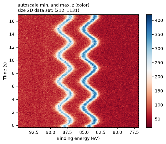
Load time- and energy-resolved XPS data from CSV files. Unlike the synthetic dataset in 01_basic_fitting, this is real, measured data: Au 4f spectra acquired at beamline 9.3.1 of the Advanced Light Source, with a ±1 V sample-bias modulation at 0.25 Hz switched on at t = 0. There are no “truth” files; instead, the known physics of the Au 4f doublet and the applied modulation anchor the fit (see §4). The 2D data array is [time, energy], i.e. rows are time, columns are energy.
# Create project (YAML model files are resolved relative to this path)
project = trspecfit.Project(path=Path.cwd())

# Directory containing data files
data_folder = 'data'

# Add file to project
file = trspecfit.File(
    parent_project=project,
    path=data_folder,
    data=np.loadtxt(project.path / data_folder / 'data.csv', delimiter=','),
    energy=np.loadtxt(project.path / data_folder / 'energy.csv'),
    time=np.loadtxt(project.path / data_folder / 'time.csv')
)
1.2 Inspect Data#
Two overlapping GLP peaks (the spin-orbit doublet) sit on a Shirley background. After t = 0 the doublet position oscillates in time.
# Visualize full dataset
file.describe()
File: data [path: data]
1.3 Define Fitting Region#
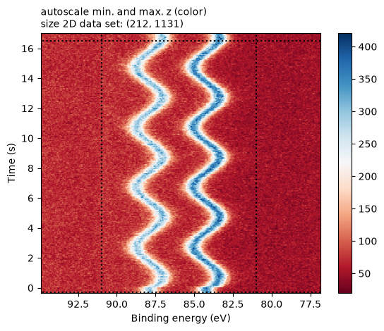
Set energy and time limits for the fits. They appear as black, dotted lines in the plot.
# Set fitting limits (absolute values)
file.set_fit_limits(
    energy_limits=[91, 81],  # Energy range in eV (descending binding-energy axis)
    time_limits=[-0.3, 16.5]  # Time range
)
2. Fit Baseline with Linked Parameters#
2.1 Define Baseline Spectrum#
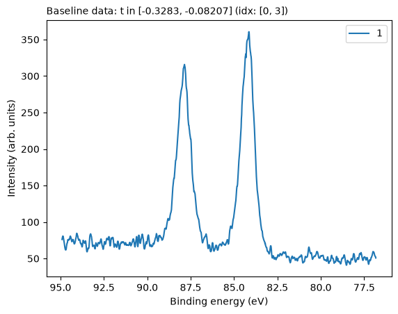
Extract the ground-state spectrum by averaging the pre-perturbation time slices.
# Define baseline using time indices
# Indices 0-3 are the four slices before t = 0; the modulation starts at t = 0,
# so the slice at index 4 (t ~ 0) must not bleed into the baseline.
file.define_baseline(
    time_start=0,
    time_stop=3,
    time_type='ind'  # Use indices (or 'abs' for absolute time values)
)
2.2 The Baseline Model and Its Linked Parameters#
The model is defined in models_energy.yaml. The first peak (GLP_01) is fit normally. The second peak (GLP_02) is linked to the first through expressions instead of being given its own free parameters:
GLP:                       # GLP_01 -- fit freely
  A:  [200, True, 0, 1000]
  x0: [84.5, True, 82, 88]
  F:  [1.0, True, 0.75, 2.5]
  m:  [0.3, True, 0, 1]
GLP:                       # GLP_02 -- derived from GLP_01
  A:  ["3/4*GLP_01_A"]     # intensity ratio
  x0: ["GLP_01_x0 + 3.67"] # energy splitting (eV)
  F:  ["GLP_01_F"]         # shared width
  m:  ["GLP_01_m"]         # shared mixing
How to reference a parameter: use its full name {component}_{NN}_{parameter}, where NN is the two-digit, auto-assigned component number (e.g. GLP_01_A). There is no $ prefix.
What you can write in an expression
Pattern |
Example |
Notes |
|---|---|---|
Copy |
|
tie a parameter to another |
Scale / ratio |
|
fixed intensity ratio |
Offset |
|
fixed splitting |
Several parameters |
|
arithmetic |
Fan-out |
many peaks → one base |
static scaling of a shared base |
Reference a dynamic base |
|
the expression inherits the dynamics (see §3) |
What you cannot do
Chain through a time- or profile-varying parameter (
C → B → A_dynamic). Reference the varying base directly instead.Self / circular references.
Add dynamics or a profile to an expression parameter — add them to the base parameter it references.
See docs/design/supported_models.md for the full contract.
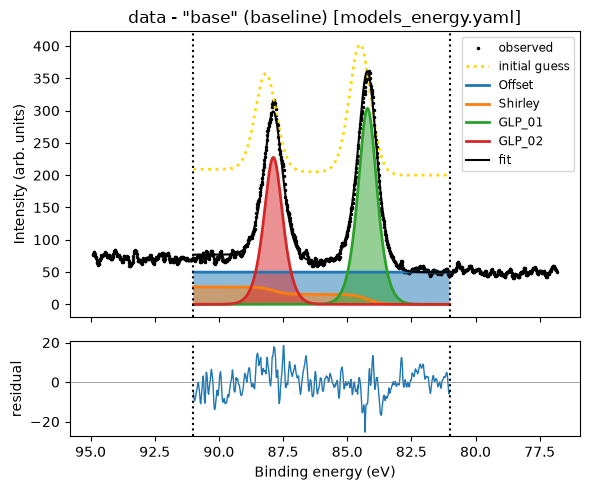
During the fit, the values of all fixed parameters (vary=False) and all expression parameters are derived automatically; only GLP_01’s free parameters and the background are optimized.
# Load baseline model
file.load_model(
    model_yaml='models_energy.yaml',
    model_info='base'
)

# Inspect model structure -- note the expr column for the GLP_02 parameters
# (detail=1 also plots the initial guess)
file.describe_model(model_info='base', detail=0)
Loading model to describe energy- (and time-)dependent data: base
model name: base
function: Offset from trspecfit.functions.energy
function: Shirley from trspecfit.functions.energy
function: GLP from trspecfit.functions.energy
function: GLP from trspecfit.functions.energy
all lmfit.Parameters() [flattened and sorted alphabetically]:
Name                 Value      Min      Max   Stderr     Vary     Expr Brute_Step
GLP_01_A               200        0     1000     None     True     None     None
GLP_01_F                 1     0.75      2.5     None     True     None     None
GLP_01_m               0.3        0        1     None     True     None     None
GLP_01_x0             84.5       82       88     None     True     None     None
GLP_02_A               150     -inf      inf     None    False 3/4*GLP_01_A     None
GLP_02_F                 1     -inf      inf     None    False GLP_01_F     None
GLP_02_m               0.3     -inf      inf     None    False GLP_01_m     None
GLP_02_x0            88.17     -inf      inf     None    False GLP_01_x0 + 3.67     None
Offset_y0              200        0      500     None     True     None     None
Shirley_pShirley    0.0004    1e-09        1     None     True     None     None
# Fit baseline model to data
# stages=1: single optimization
# stages=2: simplex pass, then leastsq refinement
file.fit_baseline(
    model_name='base',
    stages=2,
    try_ci=0  # skip confidence intervals: see 12_uncertainty_mcmc
)
Time initialize: 1.9311904907226562e-05 s

Results global minumum fit (method=Nelder):
[[Variables]]
    Offset_y0:         49.8686218 +/- 0.55008686 (1.10%) (init = 200)
    Shirley_pShirley:  8.2742e-04 +/- 2.1098e-05 (2.55%) (init = 0.0004)
    GLP_01_A:          303.359715 +/- 1.29373342 (0.43%) (init = 200)
    GLP_01_x0:         84.2079279 +/- 0.00149252 (0.00%) (init = 84.5)
    GLP_01_F:          0.90331115 +/- 0.00582955 (0.65%) (init = 1)
    GLP_01_m:          0.62597716 +/- 0.02136005 (3.41%) (init = 0.3)
    GLP_02_A:          227.519786 +/- 0.97030007 (0.43%) == '3/4*GLP_01_A'
    GLP_02_x0:         87.8779279 +/- 0.00149252 (0.00%) == 'GLP_01_x0 + 3.67'
    GLP_02_F:          0.90331115 +/- 0.00582955 (0.65%) == 'GLP_01_F'
    GLP_02_m:          0.62597716 +/- 0.02136005 (3.41%) == 'GLP_01_m'
[[Correlations]] (unreported correlations are < 0.100)
    C(GLP_01_F, GLP_01_m)          = -0.6797
    C(GLP_01_A, GLP_01_F)          = -0.6535
    C(GLP_01_A, GLP_01_m)          = +0.6097
    C(Offset_y0, Shirley_pShirley) = -0.5478
    C(Offset_y0, GLP_01_m)         = -0.3969
    C(Offset_y0, GLP_01_A)         = -0.3555
    C(Shirley_pShirley, GLP_01_x0) = -0.2659
    C(Offset_y0, GLP_01_x0)        = +0.1822
Time fit (global minimum): 0.2511429786682129 s

Results local optimization fit (method=leastsq):
[[Variables]]
    Offset_y0:         49.8687327 +/- 0.54666533 (1.10%) (init = 200)
    Shirley_pShirley:  8.2743e-04 +/- 2.1103e-05 (2.55%) (init = 0.0004)
    GLP_01_A:          303.358740 +/- 1.29232819 (0.43%) (init = 200)
    GLP_01_x0:         84.2079271 +/- 0.00148971 (0.00%) (init = 84.5)
    GLP_01_F:          0.90331475 +/- 0.00583894 (0.65%) (init = 1)
    GLP_01_m:          0.62595688 +/- 0.02110272 (3.37%) (init = 0.3)
    GLP_02_A:          227.519055 +/- 0.96924614 (0.43%) == '3/4*GLP_01_A'
    GLP_02_x0:         87.8779271 +/- 0.00148971 (0.00%) == 'GLP_01_x0 + 3.67'
    GLP_02_F:          0.90331475 +/- 0.00583894 (0.65%) == 'GLP_01_F'
    GLP_02_m:          0.62595688 +/- 0.02110272 (3.37%) == 'GLP_01_m'
[[Correlations]] (unreported correlations are < 0.100)
    C(GLP_01_F, GLP_01_m)          = -0.6817
    C(GLP_01_A, GLP_01_F)          = -0.6536
    C(GLP_01_A, GLP_01_m)          = +0.6086
    C(Offset_y0, Shirley_pShirley) = -0.5499
    C(Offset_y0, GLP_01_m)         = -0.3796
    C(Offset_y0, GLP_01_A)         = -0.3440
    C(Shirley_pShirley, GLP_01_x0) = -0.2689
    C(Offset_y0, GLP_01_x0)        = +0.1672
Time fit (local optimization): 0.006585836410522461 s
Time elapsed for baseline fit: 00.542(ss.ms)
| name | value | standard error | relative error | initial value | min | max | vary | expression |
|---|---|---|---|---|---|---|---|---|
| Offset_y0 | 49.8687327 | 0.54666533 | (1.10%) | 200.0 | 0.00000000 | 500.000000 | True | |
| Shirley_pShirley | 8.2743e-04 | 2.1103e-05 | (2.55%) | 0.0004 | 1.0000e-09 | 1.00000000 | True | |
| GLP_01_A | 303.358740 | 1.29232819 | (0.43%) | 200.0 | 0.00000000 | 1000.00000 | True | |
| GLP_01_x0 | 84.2079271 | 0.00148971 | (0.00%) | 84.5 | 82.0000000 | 88.0000000 | True | |
| GLP_01_F | 0.90331475 | 0.00583894 | (0.65%) | 1.0 | 0.75000000 | 2.50000000 | True | |
| GLP_01_m | 0.62595688 | 0.02110272 | (3.37%) | 0.3 | 0.00000000 | 1.00000000 | True | |
| GLP_02_A | 227.519055 | 0.96924614 | (0.43%) | 150.0 | -inf | inf | False | 3/4*GLP_01_A |
| GLP_02_x0 | 87.8779271 | 0.00148971 | (0.00%) | 88.17 | -inf | inf | False | GLP_01_x0 + 3.67 |
| GLP_02_F | 0.90331475 | 0.00583894 | (0.65%) | 1.0 | -inf | inf | False | GLP_01_F |
| GLP_02_m | 0.62595688 | 0.02110272 | (3.37%) | 0.3 | -inf | inf | False | GLP_01_m |
2.3 Confirm the Linked Parameters#
GLP_02 was never fit independently — its parameters are computed from GLP_01 via the expressions above. Reading the results back shows the fitted base values at full precision with their uncertainties, and below each the derived GLP_02 value with the expression that produced it: the intensity ratio is exactly 3/4 and the splitting exactly 3.67 eV, with peak 2 carrying no free parameters of its own.
# Read the linked parameters back from the baseline fit results
res = file.get_parameters(fit_type='baseline').set_index('name')

# fitted base parameter (full precision, with stderr), then the value derived
# from it through the expression
for base, derived in (('GLP_01_A', 'GLP_02_A'), ('GLP_01_x0', 'GLP_02_x0')):
    v1, e1 = res.loc[base, 'value'], res.loc[base, 'stderr']
    v2, expr = res.loc[derived, 'value'], res.loc[derived, 'expr']
    print(f'{base:9} = {v1:12.6f} +/- {e1:.6f}   (fitted)')
    print(f'{derived:9} = {v2:12.6f}   = {expr}   (derived)')

A1, A2 = res.loc['GLP_01_A', 'value'], res.loc['GLP_02_A', 'value']
x1, x2 = res.loc['GLP_01_x0', 'value'], res.loc['GLP_02_x0', 'value']
print(f'\nA2 / A1 = {A2 / A1:.6f}      (3/4 exactly)')
print(f'x2 - x1 = {x2 - x1:.6f} eV   (3.67 exactly)')
GLP_01_A  =   303.358740 +/- 1.292328   (fitted)
GLP_02_A  =   227.519055   = 3/4*GLP_01_A   (derived)
GLP_01_x0 =    84.207927 +/- 0.001490   (fitted)
GLP_02_x0 =    87.877927   = GLP_01_x0 + 3.67   (derived)

A2 / A1 = 0.750000      (3/4 exactly)
x2 - x1 = 3.670000 eV   (3.67 exactly)
3. Global 2D Fitting with an Inherited Dynamic Link#
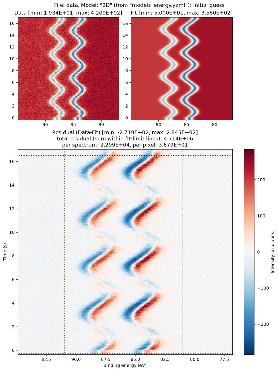
Now fit the whole dataset at once and let the first peak’s position move in time. We attach a time law (sine_wave from models_time.yaml) to GLP_01_x0.
The key point: GLP_02_x0 is defined as "GLP_01_x0 + 3.67". Because it references the now time-dependent GLP_01_x0 directly, the second peak’s position inherits the oscillation automatically — it tracks peak 1 at a fixed 3.67 eV offset, with no extra parameters. (This works precisely because the expression points at the dynamic base directly; chaining through another expression would not be allowed.)
Why global? Fitting all time points together with a single time law constrains the dynamics across the whole dataset, giving far fewer free parameters and more robust results than fitting each slice independently.
# Load 2D model (same linked doublet; pinned parameters take the baseline result)
file.load_model(
    model_yaml='models_energy.yaml',
    model_info='2D'
)

file.describe_model(model_info='2D', detail=0)
Loading model to describe energy- (and time-)dependent data: 2D
model name: 2D
function: Offset from trspecfit.functions.energy
function: Shirley from trspecfit.functions.energy
function: GLP from trspecfit.functions.energy
function: GLP from trspecfit.functions.energy
all lmfit.Parameters() [flattened and sorted alphabetically]:
Name                 Value      Min      Max   Stderr     Vary     Expr Brute_Step
GLP_01_A               300     -inf      inf     None    False     None     None
GLP_01_F                 1     -inf      inf     None    False     None     None
GLP_01_m               0.3     -inf      inf     None    False     None     None
GLP_01_x0             84.5       82       88     None     True     None     None
GLP_02_A               225     -inf      inf     None    False 3/4*GLP_01_A     None
GLP_02_F                 1     -inf      inf     None    False GLP_01_F     None
GLP_02_m               0.3     -inf      inf     None    False GLP_01_m     None
GLP_02_x0            88.17     -inf      inf     None    False GLP_01_x0 + 3.67     None
Offset_y0               50     -inf      inf     None    False     None     None
Shirley_pShirley    0.0008     -inf      inf     None    False     None     None
# Attach a sine-wave time law to the first peak's position.
# GLP_02_x0 = "GLP_01_x0 + 3.67" will inherit this oscillation automatically.
file.add_time_dependence(
    target_model='2D',
    target_parameter='GLP_01_x0',
    dynamics_yaml='models_time.yaml',
    dynamics_model='sine_wave',
)

print("\n=== Model with Time Dependence ===")
# detail=1 also plots the model at its initial guess
file.describe_model(model_info='2D', detail=1)
Loading model to describe time-dependence of a model parameter: GLP_01_x0 of sine_wave model

=== Model with Time Dependence ===
model name: 2D
function: Offset from trspecfit.functions.energy
function: Shirley from trspecfit.functions.energy
function: GLP from trspecfit.functions.energy
function: GLP from trspecfit.functions.energy
all lmfit.Parameters() [flattened and sorted alphabetically]:
Name                        Value      Min      Max   Stderr     Vary     Expr Brute_Step
GLP_01_A                      300     -inf      inf     None    False     None     None
GLP_01_F                        1     -inf      inf     None    False     None     None
GLP_01_m                      0.3     -inf      inf     None    False     None     None
GLP_01_x0                    84.5       82       88     None     True     None     None
GLP_01_x0_sinFun_01_A          -1       -5        5     None     True     None     None
GLP_01_x0_sinFun_01_f        0.25    0.001       10     None     True     None     None
GLP_01_x0_sinFun_01_phi         0    -0.75     0.75     None     True     None     None
GLP_01_x0_sinFun_01_t0          0     -inf      inf     None    False     None     None
GLP_02_A                      225     -inf      inf     None    False 3/4*GLP_01_A     None
GLP_02_F                        1     -inf      inf     None    False GLP_01_F     None
GLP_02_m                      0.3     -inf      inf     None    False GLP_01_m     None
GLP_02_x0                   88.17     -inf      inf     None    False GLP_01_x0 + 3.67     None
Offset_y0                      50     -inf      inf     None    False     None     None
Shirley_pShirley           0.0008     -inf      inf     None    False     None     None
# Perform global 2D fit
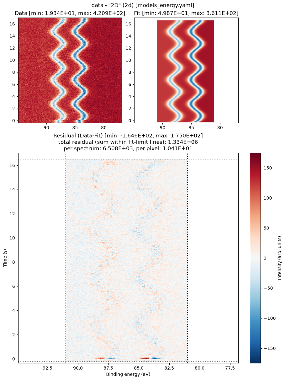
file.fit_2d(
    model_name='2D',
    stages=2,
    try_ci=0  # skip confidence intervals: see 12_uncertainty_mcmc
)
Time initialize: 1.9788742065429688e-05 s

Results global minumum fit (method=Nelder):
[[Variables]]
    Offset_y0:                49.86873 (fixed)
    Shirley_pShirley:         0.0008274333 (fixed)
    GLP_01_A:                 303.3587 (fixed)
    GLP_01_x0:                84.2099108 +/- 2.2906e-04 (0.00%) (init = 84.20793)
    GLP_01_x0_sinFun_01_A:   -0.84379986 +/- 3.2402e-04 (0.04%) (init = -1)
    GLP_01_x0_sinFun_01_f:    0.25016566 +/- 1.3034e-05 (0.01%) (init = 0.25)
    GLP_01_x0_sinFun_01_phi:  0.39851754 +/- 7.9444e-04 (0.20%) (init = 0)
    GLP_01_x0_sinFun_01_t0:   0 (fixed)
    GLP_01_F:                 0.9033147 (fixed)
    GLP_01_m:                 0.6259569 (fixed)
    GLP_02_A:                 227.519055 +/- 0.00000000 (0.00%) == '3/4*GLP_01_A'
    GLP_02_x0:                87.8799108 +/- 2.2906e-04 (0.00%) == 'GLP_01_x0 + 3.67'
    GLP_02_F:                 0.90331475 +/- 0.00000000 (0.00%) == 'GLP_01_F'
    GLP_02_m:                 0.62595688 +/- 0.00000000 (0.00%) == 'GLP_01_m'
[[Correlations]] (unreported correlations are < 0.100)
    C(GLP_01_x0_sinFun_01_f, GLP_01_x0_sinFun_01_phi) = -0.8759
    C(GLP_01_x0, GLP_01_x0_sinFun_01_f)               = +0.1238
Time fit (global minimum): 6.673462629318237 s

Results local optimization fit (method=leastsq):
[[Variables]]
    Offset_y0:                49.86873 (fixed)
    Shirley_pShirley:         0.0008274333 (fixed)
    GLP_01_A:                 303.3587 (fixed)
    GLP_01_x0:                84.2099108 +/- 2.2552e-04 (0.00%) (init = 84.20793)
    GLP_01_x0_sinFun_01_A:   -0.84379986 +/- 3.1905e-04 (0.04%) (init = -1)
    GLP_01_x0_sinFun_01_f:    0.25016566 +/- 1.2673e-05 (0.01%) (init = 0.25)
    GLP_01_x0_sinFun_01_phi:  0.39851754 +/- 7.6936e-04 (0.19%) (init = 0)
    GLP_01_x0_sinFun_01_t0:   0 (fixed)
    GLP_01_F:                 0.9033147 (fixed)
    GLP_01_m:                 0.6259569 (fixed)
    GLP_02_A:                 227.519055 +/- 0.00000000 (0.00%) == '3/4*GLP_01_A'
    GLP_02_x0:                87.8799108 +/- 2.2552e-04 (0.00%) == 'GLP_01_x0 + 3.67'
    GLP_02_F:                 0.90331475 +/- 0.00000000 (0.00%) == 'GLP_01_F'
    GLP_02_m:                 0.62595688 +/- 0.00000000 (0.00%) == 'GLP_01_m'
[[Correlations]] (unreported correlations are < 0.100)
    C(GLP_01_x0_sinFun_01_f, GLP_01_x0_sinFun_01_phi) = -0.8707
    C(GLP_01_x0, GLP_01_x0_sinFun_01_f)               = +0.1141
Time fit (local optimization): 0.13016819953918457 s
Time elapsed for 2D model fit: 07.739(ss.ms)
| name | value | standard error | relative error | initial value | min | max | vary | expression |
|---|---|---|---|---|---|---|---|---|
| Offset_y0 | 49.8687327 | 0.00000000 | (0.00%) | 49.86873267889691 | -inf | inf | False | |
| Shirley_pShirley | 8.2743e-04 | 0.00000000 | (0.00%) | 0.0008274332769612655 | -inf | inf | False | |
| GLP_01_A | 303.358740 | 0.00000000 | (0.00%) | 303.35874012852395 | -inf | inf | False | |
| GLP_01_x0 | 84.2099108 | 2.2552e-04 | (0.00%) | 84.20792709553795 | 82.0000000 | 88.0000000 | True | |
| GLP_01_x0_sinFun_01_A | -0.84379986 | 3.1905e-04 | (0.04%) | -1.0 | -5.00000000 | 5.00000000 | True | |
| GLP_01_x0_sinFun_01_f | 0.25016566 | 1.2673e-05 | (0.01%) | 0.25 | 1.0000e-03 | 10.0000000 | True | |
| GLP_01_x0_sinFun_01_phi | 0.39851754 | 7.6936e-04 | (0.19%) | 0.0 | -0.75000000 | 0.75000000 | True | |
| GLP_01_x0_sinFun_01_t0 | 0.00000000 | 0.00000000 | 0.0 | -inf | inf | False | ||
| GLP_01_F | 0.90331475 | 0.00000000 | (0.00%) | 0.9033147491163926 | -inf | inf | False | |
| GLP_01_m | 0.62595688 | 0.00000000 | (0.00%) | 0.6259568757143346 | -inf | inf | False | |
| GLP_02_A | 227.519055 | 0.00000000 | (0.00%) | 227.51905509639295 | -inf | inf | False | 3/4*GLP_01_A |
| GLP_02_x0 | 87.8799108 | 2.2552e-04 | (0.00%) | 87.87792709553796 | -inf | inf | False | GLP_01_x0 + 3.67 |
| GLP_02_F | 0.90331475 | 0.00000000 | (0.00%) | 0.9033147491163926 | -inf | inf | False | GLP_01_F |
| GLP_02_m | 0.62595688 | 0.00000000 | (0.00%) | 0.6259568757143346 | -inf | inf | False | GLP_01_m |
4. Inspect the Fit Results#
file.get_parameters(fit_type='2d') returns a pandas.DataFrame with one row per parameter. The first peak’s position now carries the sine-wave dynamics parameters (GLP_01_x0_sinFun_01_*), while GLP_02_x0 keeps its expression in the expr column. Peak 2 therefore follows peak 1 plus 3.67 eV at every time point, with no free parameters of its own.
Since this is measured data, the fit is checked against the experiment and the literature instead of a truth file. The fitted modulation frequency (f ≈ 0.2502 Hz) recovers the applied 0.25 Hz bias modulation. The fitted 4f7/2 position (≈ 84.2 eV) lands near the tabulated Au 4f7/2 binding energy of 84.0 eV. The 3.67 eV splitting and 3:4 intensity ratio enforced by the expressions are themselves the literature values for the Au 4f doublet. The fitted oscillation amplitude (≈ 0.84 eV) is smaller than the ±1 V drive: the sample’s response to the bias is damped, while the frequency carries over unchanged.
For more on accessing fit results and metadata, see 10_model_comparison.
file.get_parameters(fit_type='2d')
| name | value | stderr | init_value | min | max | vary | expr | |
|---|---|---|---|---|---|---|---|---|
| 0 | Offset_y0 | 49.868733 | 0.000000 | 49.868733 | -inf | inf | False | NaN |
| 1 | Shirley_pShirley | 0.000827 | 0.000000 | 0.000827 | -inf | inf | False | NaN |
| 2 | GLP_01_A | 303.358740 | 0.000000 | 303.358740 | -inf | inf | False | NaN |
| 3 | GLP_01_x0 | 84.209911 | 0.000226 | 84.207927 | 82.000 | 88.00 | True | NaN |
| 4 | GLP_01_x0_sinFun_01_A | -0.843800 | 0.000319 | -1.000000 | -5.000 | 5.00 | True | NaN |
| 5 | GLP_01_x0_sinFun_01_f | 0.250166 | 0.000013 | 0.250000 | 0.001 | 10.00 | True | NaN |
| 6 | GLP_01_x0_sinFun_01_phi | 0.398518 | 0.000769 | 0.000000 | -0.750 | 0.75 | True | NaN |
| 7 | GLP_01_x0_sinFun_01_t0 | 0.000000 | 0.000000 | 0.000000 | -inf | inf | False | NaN |
| 8 | GLP_01_F | 0.903315 | 0.000000 | 0.903315 | -inf | inf | False | NaN |
| 9 | GLP_01_m | 0.625957 | 0.000000 | 0.625957 | -inf | inf | False | NaN |
| 10 | GLP_02_A | 227.519055 | 0.000000 | 227.519055 | -inf | inf | False | 3/4*GLP_01_A |
| 11 | GLP_02_x0 | 87.879911 | 0.000226 | 87.877927 | -inf | inf | False | GLP_01_x0 + 3.67 |
| 12 | GLP_02_F | 0.903315 | 0.000000 | 0.903315 | -inf | inf | False | GLP_01_F |
| 13 | GLP_02_m | 0.625957 | 0.000000 | 0.625957 | -inf | inf | False | GLP_01_m |
Tips for Dependent Parameters#
Writing expressions
Reference a parameter by its full name
{component}_{NN}_{parameter}(e.g.GLP_01_A); there is no$prefix.Use arithmetic (
+ - * / ** %); expressions are evaluated by the same safe evaluator lmfit uses.Common patterns: spin-orbit splitting, vibrational progressions, shared backgrounds, fixed intensity ratios.
Allowed vs. not allowed
Supported: link to other top-level parameters; static fan-out from a shared base; reference a time-dependent or profiled base directly (the expression inherits the variation).
Not supported: chain through a varying parameter (
C → B → A_dynamic) — reference the base directly. No self / circular references. Don’t attach dynamics or profiles to an expression parameter.Source of truth:
docs/design/supported_models.md.
Strategy
Fewer free parameters → more robust, faster fits. Use links to encode known physics.
Fit the baseline first: the 2D model pins its line-shape and background parameters to the baseline result and fits only the dynamics.
Add a time law to the base parameter and let the linked parameters inherit it.
Next Steps#
Datasets with multiple sub-cycles:
03_multi_cycle_dynamicsParameters that vary along an auxiliary axis:
04_parameter_profilesUncertainty estimation (MCMC):
12_uncertainty_mcmcSave, load, and export fits:
11_save_load_export
Model files#
The YAML files next to this notebook, as shipped with the example.
models_energy.yaml#
# Use these models to describe the energy-dependent data
# For available functions see: /src/trspecfit/functions/energy.py

# Ground state (most parameters should be able to vary)
# The two GLP peaks form a spin-orbit doublet (auto-numbered during model loading):
# GLP_02 is fully derived from GLP_01 via expressions (no free parameters of its own).
base:
    Offset:
      y0: [200, True, 0, 500]
    Shirley:
        pShirley: [4.0E-4, True, 1.0E-9, 1.0]
    GLP:                       # GLP_01 -- the fit-varying peak
      A: [200, True, 0, 1000]
      x0: [84.5, True, 82, 88]
      F: [1.0, True, 0.75, 2.5]
      m: [0.3, True, 0, 1]
    GLP:                       # GLP_02 -- derived from GLP_01
      A: ["3/4*GLP_01_A"]      # fixed intensity ratio (3:4)
      x0: ["GLP_01_x0 + 3.67"] # fixed energy splitting (eV)
      F: ["GLP_01_F"]          # shared width
      m: ["GLP_01_m"]          # shared mixing

# 2D model fit (pinned parameters will be set to "base" Model fit result values).
# Same linked doublet; add_time_dependence() attaches a time law to GLP_01_x0 and
# GLP_02_x0 inherits it through its expression.
2D:
    Offset:
      y0: [50, False]
    Shirley:
        pShirley: [8.0E-4, False]
    GLP:                       # GLP_01 -- position becomes time-dependent
      A: [300, False]
      x0: [84.5, True, 82, 88]
      F: [1.0, False]
      m: [0.3, False]
    GLP:                       # GLP_02 -- inherits GLP_01's dynamics via x0 expr
      A: ["3/4*GLP_01_A"]      # fixed intensity ratio (3:4)
      x0: ["GLP_01_x0 + 3.67"] # fixed energy splitting (eV)
      F: ["GLP_01_F"]          # shared width
      m: ["GLP_01_m"]          # shared mixing
models_time.yaml#
# Use these models to add time-dependence to a parameter in a 2D model
# For available functions see: /src/trspecfit/functions/time.py

sine_wave:
    sinFun:
        A: [-1, True, -5, 5]
        f: [0.25, True, 1E-3, 10]
        phi: [0, True, -0.75, 0.75]
        t0: [0, False]
project.yaml#
# Project configuration for trspecfit dependent_parameters example

# Display settings (general verbosity)
show_output: 1  # 0: silent/API mode, 1: interactive/notebook mode

# Axis labels
e_label: 'Binding energy (eV)' # x -> energy
t_label: 'Time (s)' # y -> time
z_label: 'Intensity (arb. units)' # z -> intensity

# Plot settings
x_dir: 'rev'  # def(ault) or rev(erse)
x_type: 'lin'  # lin or log
y_dir: 'def'  # def(ault) or rev(erse)
y_type: 'lin'  # lin or log
z_colormap: 'RdBu' # colormap in 2D plots
z_type: 'lin'  # lin or log (2D plots)
dpi_plt: 100 # figure display dpi
dpi_save: 300 # figure save dpi
res_mult: 5 # residual multiplier in figures