Generate Synthetic Data for Shared-Parameter Fitting#
Generate multiple datasets that share the same spectral model but differ in the amplitude of the time-dependent peak shift. This simulates a common experimental scenario where identical samples are measured at different pump fluences or excitation intensities.
Ground truth model:
GLP peak + linear background (
LinBack)Time dependence: exponential shift of peak position (
expFun+gaussCONVIRF)6 datasets with
expFun A:[5, 2, 1, 0.5, 0.2, 0.1]All other parameters identical across files
import os
import numpy as np
import trspecfit
1. Define Ground Truth Model#
Build a 2D model (energy + time) from YAML files. The models_energy_truth.yaml
and models_time_truth.yaml files define the ground truth parameters.
project = trspecfit.Project(path=os.getcwd())

energy = np.arange(0, 20, 0.1)
time = np.concatenate([
    np.arange(-20, 5, 0.5),   # fine steps around t0
    np.arange(5, 100, 2.0),   # coarser for the decay tail
])

file = trspecfit.File(
    parent_project=project,
    energy=energy,
    time=time,
)

# Load energy model
file.load_model(
    model_yaml='models_energy_truth.yaml',
    model_info='single_peak',
)

# Add time dependence to peak position
file.add_time_dependence(
    target_model='single_peak',
    target_parameter='GLP_01_x0',
    dynamics_yaml='models_time_truth.yaml',
    dynamics_model=['MonoExpPosIRF'],
)

file.describe_model()
Config file <repo>/examples/fitting_workflows/21_multi_file_shared_fit/data/project.yaml not found, using defaults
Loading model to describe energy- (and time-)dependent data: single_peak
Loading model to describe time-dependence of a model parameter: GLP_01_x0 of MonoExpPosIRF model
model name: single_peak
function: LinBack from trspecfit.functions.energy
function: GLP from trspecfit.functions.energy
all lmfit.Parameters() [flattened and sorted alphabetically]:
Name                        Value      Min      Max   Stderr     Vary     Expr Brute_Step
GLP_01_A                       10        5       15     None     True     None     None
GLP_01_F                        1     0.75      2.5     None     True     None     None
GLP_01_m                      0.3        0        1     None     True     None     None
GLP_01_x0                      10        5       15     None     True     None     None
GLP_01_x0_expFun_01_A           5        0       15     None     True     None     None
GLP_01_x0_expFun_01_t0          0     -inf      inf     None    False     None     None
GLP_01_x0_expFun_01_tau        50        1      100     None     True     None     None
GLP_01_x0_gaussCONV_SD          3    1e-06       10     None     True     None     None
LinBack_b                       0       -5        5     None     True     None     None
LinBack_m                     0.4       -1        1     None     True     None     None
LinBack_xStart                  0     -inf      inf     None    False     None     None
LinBack_xStop                  20     -inf      inf     None    False     None     None
2. Generate Datasets at Different Shift Amplitudes#
Each amplitude is its own dynamics entry in models_time_truth.yaml (the YAML
is the source of truth; a variant is another entry). For each one, reload the
energy model, attach that entry, simulate noisy data, and save to CSV. The axes
are shared across all files.
amplitudes = [5, 2, 1, 0.5, 0.2, 0.1]

# Save shared axes (once)
np.savetxt('energy.csv', energy)
np.savetxt('time.csv', time)

for i, amp in enumerate(amplitudes, start=1):
    # The shift amplitude is a dynamics entry of its own: reload the
    # energy model and attach the entry for this amplitude
    file.load_model(
        model_yaml='models_energy_truth.yaml',
        model_info='single_peak',
    )
    file.add_time_dependence(
        target_model='single_peak',
        target_parameter='GLP_01_x0',
        dynamics_yaml='models_time_truth.yaml',
        dynamics_model=[f'MonoExpPosIRF_A{amp:g}'.replace('.', 'p')],
    )
    model = file.model_active

    # Simulate with photon counting noise
    sim = trspecfit.Simulator(
        model=model,
        detection='photon_counting',
        counts_per_delay=5000,
        seed=42 + i,
    )
    _clean, noisy, _noise = sim.simulate_2d()

    # Save data
    np.savetxt(f'data_{i}.csv', noisy, delimiter=',')
    print(f'data_{i}.csv  |  expFun A = {amp:6.3f}  |  shape {noisy.shape}')
Loading model to describe energy- (and time-)dependent data: single_peak
Loading model to describe time-dependence of a model parameter: GLP_01_x0 of MonoExpPosIRF_A5 model
data_1.csv  |  expFun A =  5.000  |  shape (98, 200)
Loading model to describe energy- (and time-)dependent data: single_peak
Loading model to describe time-dependence of a model parameter: GLP_01_x0 of MonoExpPosIRF_A2 model
data_2.csv  |  expFun A =  2.000  |  shape (98, 200)
Loading model to describe energy- (and time-)dependent data: single_peak
Loading model to describe time-dependence of a model parameter: GLP_01_x0 of MonoExpPosIRF_A1 model
data_3.csv  |  expFun A =  1.000  |  shape (98, 200)
Loading model to describe energy- (and time-)dependent data: single_peak
Loading model to describe time-dependence of a model parameter: GLP_01_x0 of MonoExpPosIRF_A0p5 model
data_4.csv  |  expFun A =  0.500  |  shape (98, 200)
Loading model to describe energy- (and time-)dependent data: single_peak
Loading model to describe time-dependence of a model parameter: GLP_01_x0 of MonoExpPosIRF_A0p2 model
data_5.csv  |  expFun A =  0.200  |  shape (98, 200)
Loading model to describe energy- (and time-)dependent data: single_peak
Loading model to describe time-dependence of a model parameter: GLP_01_x0 of MonoExpPosIRF_A0p1 model
data_6.csv  |  expFun A =  0.100  |  shape (98, 200)
<cell>:10: UserWarning: Model "single_peak" already exists on file 'test' — replacing the live model object. Completed fits are unaffected (they are kept in the fit history).
  file.load_model(
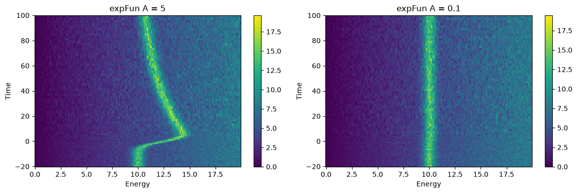
3. Quick Visual Check#
Plot the strongest and weakest datasets side by side.
import matplotlib.pyplot as plt

fig, axes = plt.subplots(1, 2, figsize=(12, 4))

d1 = np.loadtxt('data_1.csv', delimiter=',')
d6 = np.loadtxt('data_6.csv', delimiter=',')

im0 = axes[0].pcolormesh(energy, time, d1, shading='auto')
axes[0].set_title(f'expFun A = {amplitudes[0]}')
axes[0].set_xlabel('Energy')
axes[0].set_ylabel('Time')
plt.colorbar(im0, ax=axes[0])

im1 = axes[1].pcolormesh(energy, time, d6, shading='auto')
axes[1].set_title(f'expFun A = {amplitudes[-1]}')
axes[1].set_xlabel('Energy')
axes[1].set_ylabel('Time')
plt.colorbar(im1, ax=axes[1])

plt.tight_layout()
plt.show()
Ground Truth Parameters#
Parameter |
Value |
Description |
|---|---|---|
|
0.4 |
Background slope |
|
0.0 |
Background intercept |
|
0 |
Background start |
|
20 |
Background stop |
|
10 |
Peak amplitude |
|
10 |
Peak center |
|
1.0 |
Peak width |
|
0.3 |
Mixing (Gauss/Lorentz) |
|
3 |
IRF width |
|
varies |
Shift amplitude |
|
50 |
Decay time constant |
|
0 |
Time zero |
Model files#
The YAML files next to this notebook, as shipped with the example.
models_energy_truth.yaml#
# ground truth model for data generation
# parameters: [value, vary, min, max]

single_peak:
    LinBack:
      m: [4E-1, True, -1, 1]
      b: [0, True, -5, 5]
      xStart: [0, False]
      xStop: [20, False]
    GLP:
      A: [10, True, 5, 15]
      x0: [10, True, 5, 15]
      F: [1.0, True, 0.75, 2.5]
      m: [0.3, True, 0, 1]
models_time_truth.yaml#
# ground truth time model for data generation

MonoExpPosIRF:
    gaussCONV:
        SD: [3, True, 1.0E-6, 10]
    expFun:
        A: [5, True, 0, 15]
        tau: [50, True, 1, 100]
        t0: [0, False]

# MonoExpPosIRF with the shift amplitude at 5: one entry per dataset
MonoExpPosIRF_A5:
    gaussCONV:
        SD: [3, True, 1.0E-6, 10]
    expFun:
        A: [5, True, 0, 15]
        tau: [50, True, 1, 100]
        t0: [0, False]

# MonoExpPosIRF with the shift amplitude at 2: one entry per dataset
MonoExpPosIRF_A2:
    gaussCONV:
        SD: [3, True, 1.0E-6, 10]
    expFun:
        A: [2, True, 0, 15]
        tau: [50, True, 1, 100]
        t0: [0, False]

# MonoExpPosIRF with the shift amplitude at 1: one entry per dataset
MonoExpPosIRF_A1:
    gaussCONV:
        SD: [3, True, 1.0E-6, 10]
    expFun:
        A: [1, True, 0, 15]
        tau: [50, True, 1, 100]
        t0: [0, False]

# MonoExpPosIRF with the shift amplitude at 0.5: one entry per dataset
MonoExpPosIRF_A0p5:
    gaussCONV:
        SD: [3, True, 1.0E-6, 10]
    expFun:
        A: [0.5, True, 0, 15]
        tau: [50, True, 1, 100]
        t0: [0, False]

# MonoExpPosIRF with the shift amplitude at 0.2: one entry per dataset
MonoExpPosIRF_A0p2:
    gaussCONV:
        SD: [3, True, 1.0E-6, 10]
    expFun:
        A: [0.2, True, 0, 15]
        tau: [50, True, 1, 100]
        t0: [0, False]

# MonoExpPosIRF with the shift amplitude at 0.1: one entry per dataset
MonoExpPosIRF_A0p1:
    gaussCONV:
        SD: [3, True, 1.0E-6, 10]
    expFun:
        A: [0.1, True, 0, 15]
        tau: [50, True, 1, 100]
        t0: [0, False]