Multi-Cycle Time-Dependent Fitting#
This notebook shows how to fit repeating, multi-phase dynamics by passing a list of models to add_time_dependence. The example system is the same as in 01_basic_fitting: a GLP peak on a linear background.
However, after t = 0 the peak position now alternates between two repeating subcycles: a negative shift that relaxes quickly and a mirrored positive shift that relaxes more slowly, all blurred by a Gaussian instrument response function (IRF).
The two rules that drive everything here:
The
dynamics_modellist. Element 0 applies globally, across all times t, and is typically used for an IRF convolution. All following elements alternate as subcycles within each repetition period. IfNis the length of thedynamics_modellist, thenN-1is the number of subcycles.The
frequencyparameter. Simply 1/T of the full repeating period, in the reciprocal units of your time axis (atimeaxis in ps makesfrequencya rate per ps, not Hz). TheN−1subcycle models split each period equally, so one subcycle lasts1/(frequency*(N-1)). Subcycles start at t = 0; everything before is baseline.
Workflow:
Select the data: load, inspect, set fit limits.
Fit the baseline (
base): ground-state spectrum from pre-trigger slices.Slice-by-slice fitting (
SbS): reveal the alternating sawtooth that motivates the multi-cycle model.Multi-cycle 2D fit (
2D): one global fit with['IRF', 'MonoExpNeg', 'MonoExpPos']repeating atfrequency=0.25.Inspect the results: compare to the known truth (
data/models_energy_truth.yaml,data/models_time_truth.yaml).
from pathlib import Path

import numpy as np
import trspecfit
1. Load and Inspect Data#
1.1 Load Data#
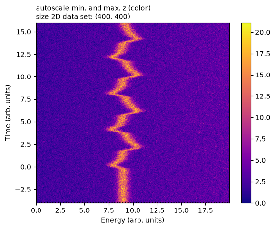
Load simulated time- and energy-resolved spectroscopy data from CSV files. The data is synthetic, generated by data/generate_data.ipynb which can be re-run to regenerate or change the data.
The 2D dataset is a stack of 1D energy spectra, one per time delay. The data array is [time, energy], i.e. rows are time, columns are energy.
# Create project
project = trspecfit.Project(path=Path.cwd())

# Directory containing data files
data_folder = 'data'

# Add file to project
file = trspecfit.File(
    parent_project=project,
    path=data_folder,
    data=np.loadtxt(project.path / data_folder / 'data.csv', delimiter=','),
    energy=np.loadtxt(project.path / data_folder / 'energy.csv'),
    time=np.loadtxt(project.path / data_folder / 'time.csv')
)
1.2 Inspect Data#
A GLP peak sits on a linear background (LinBack). After t = 0 the peak position alternates periodically: it jumps down and relaxes back (fast), then jumps up by the same amount and relaxes back (slower), repeating every 4 time units. The sharp jumps are rounded by the Gaussian IRF.
# Visualize full dataset
file.describe()
File: data [path: data]
1.3 Define Fitting Region#
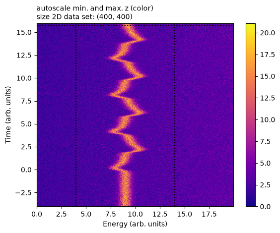
Set energy and time limits for the fits. They appear as black, dotted lines in the plot.
# Set fitting limits (absolute values)
file.set_fit_limits(
    energy_limits=[4, 14],  # Energy range
    time_limits=[-4, 15.75]  # Time range
)
2. Fit Baseline / Ground State Spectrum#
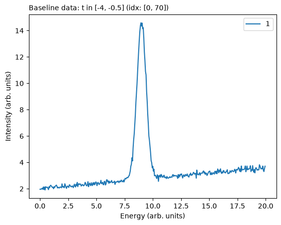
2.1 Define Baseline Spectrum#
Extract the ground-state spectrum by averaging pre-trigger time slices. The Gaussian IRF is non-causal — it bleeds the first subcycle’s onset slightly before t = 0 — so stop the baseline well before t = 0 (here at −0.5, about 3 IRF widths).
# Define baseline using absolute time values
file.define_baseline(
    time_start=-4,
    time_stop=-0.5,
    time_type='abs'  # Use absolute time values (or 'ind' for indices)
)
2.2 Fit Baseline Spectrum#
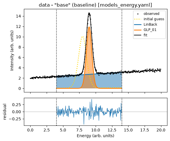
Fit the ground state spectrum leaving most fit parameters free to vary. The model is defined in models_energy.yaml.
During time-dependent fits, the values of all fixed parameters (vary=False) will be set to the baseline fit result values.
# Load baseline model
file.load_model(
    model_yaml='models_energy.yaml',
    model_info='base'
)

# Inspect model structure and parameters (detail=1 also plots the initial guess)
file.describe_model(model_info='base', detail=0)
Loading model to describe energy- (and time-)dependent data: base
model name: base
function: LinBack from trspecfit.functions.energy
function: GLP from trspecfit.functions.energy
all lmfit.Parameters() [flattened and sorted alphabetically]:
Name               Value      Min      Max   Stderr     Vary     Expr Brute_Step
GLP_01_A              10        5       15     None     True     None     None
GLP_01_F             1.5     0.75      2.5     None     True     None     None
GLP_01_m             0.3        0        1     None     True     None     None
GLP_01_x0              8        5       15     None     True     None     None
LinBack_b              0       -5        5     None     True     None     None
LinBack_m           0.01       -1        1     None     True     None     None
LinBack_xStart         0     -inf      inf     None    False     None     None
LinBack_xStop         20     -inf      inf     None    False     None     None
# Fit baseline model to data
file.fit_baseline(
    model_name='base',
    stages=2,
    try_ci=0  # skip confidence intervals: see 12_uncertainty_mcmc
)
Time initialize: 2.193450927734375e-05 s

Results global minumum fit (method=Nelder):
[[Variables]]
    LinBack_m:       0.21728593 +/- 0.01802113 (8.29%) (init = 0.01)
    LinBack_b:       0.69332964 +/- 0.17269801 (24.91%) (init = 0)
    LinBack_xStart:  0 (fixed)
    LinBack_xStop:   20 (fixed)
    GLP_01_A:        9.22630090 +/- 0.23225400 (2.52%) (init = 10)
    GLP_01_x0:       8.99315627 +/- 0.01181473 (0.13%) (init = 8)
    GLP_01_F:        1.18519950 +/- 0.03504398 (2.96%) (init = 1.5)
    GLP_01_m:        0.08995565 +/- 0.09106063 (101.23%) (init = 0.3)
[[Correlations]] (unreported correlations are < 0.100)
    C(LinBack_m, LinBack_b) = -0.9337
    C(GLP_01_F, GLP_01_m)   = +0.4042
    C(GLP_01_A, GLP_01_F)   = -0.3931
    C(LinBack_b, GLP_01_F)  = -0.1011
Time fit (global minimum): 0.15918469429016113 s

Results local optimization fit (method=leastsq):
[[Variables]]
    LinBack_m:       0.08026027 +/- 0.00291837 (3.64%) (init = 0.01)
    LinBack_b:       2.00080465 +/- 0.02805784 (1.40%) (init = 0)
    LinBack_xStart:  0 (fixed)
    LinBack_xStop:   20 (fixed)
    GLP_01_A:        11.9054139 +/- 0.04617389 (0.39%) (init = 10)
    GLP_01_x0:       9.00088919 +/- 0.00155117 (0.02%) (init = 8)
    GLP_01_F:        1.00041350 +/- 0.00442517 (0.44%) (init = 1.5)
    GLP_01_m:        0.17531026 +/- 0.04941204 (28.19%) (init = 0.3)
[[Correlations]] (unreported correlations are < 0.100)
    C(LinBack_m, LinBack_b) = -0.9361
    C(GLP_01_A, GLP_01_m)   = +0.5335
    C(GLP_01_F, GLP_01_m)   = +0.4510
    C(GLP_01_A, GLP_01_F)   = -0.1349
    C(LinBack_b, GLP_01_F)  = -0.1290
Time fit (local optimization): 0.0066204071044921875 s
Time elapsed for baseline fit: 00.421(ss.ms)
| name | value | standard error | relative error | initial value | min | max | vary |
|---|---|---|---|---|---|---|---|
| LinBack_m | 0.08026027 | 0.00291837 | (3.64%) | 0.01 | -1.00000000 | 1.00000000 | True |
| LinBack_b | 2.00080465 | 0.02805784 | (1.40%) | 0.0 | -5.00000000 | 5.00000000 | True |
| LinBack_xStart | 0.00000000 | 0.00000000 | 0.0 | -inf | inf | False | |
| LinBack_xStop | 20.0000000 | 0.00000000 | (0.00%) | 20.0 | -inf | inf | False |
| GLP_01_A | 11.9054139 | 0.04617389 | (0.39%) | 10.0 | 5.00000000 | 15.0000000 | True |
| GLP_01_x0 | 9.00088919 | 0.00155117 | (0.02%) | 8.0 | 5.00000000 | 15.0000000 | True |
| GLP_01_F | 1.00041350 | 0.00442517 | (0.44%) | 1.5 | 0.75000000 | 2.50000000 | True |
| GLP_01_m | 0.17531026 | 0.04941204 | (28.19%) | 0.3 | 0.00000000 | 1.00000000 | True |
3. Slice-by-Slice Fitting#
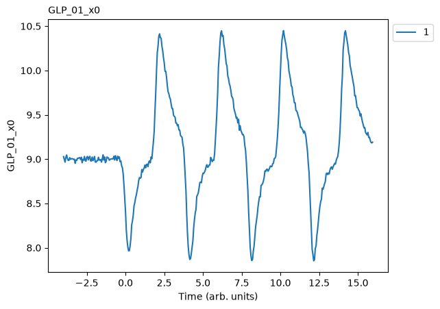
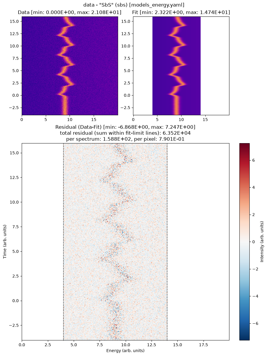
Fit each time slice independently with the peak position GLP_01_x0 as the only free parameter. The result is the position-vs-time trace without assuming any functional form — look for the alternating sawtooth: downward jumps at t = 0, 4, 8, … and upward jumps at t = 2, 6, 10, …, each relaxing back toward the baseline. That repeating two-phase pattern is what motivates a multi-cycle model; the different relaxation speeds of the two phases motivate per-subcycle time constants.
# Load Slice-by-Slice model
file.load_model(
    model_yaml='models_energy.yaml',
    model_info='SbS'
)

file.describe_model(model_info='SbS', detail=0)
Loading model to describe energy- (and time-)dependent data: SbS
model name: SbS
function: LinBack from trspecfit.functions.energy
function: GLP from trspecfit.functions.energy
all lmfit.Parameters() [flattened and sorted alphabetically]:
Name               Value      Min      Max   Stderr     Vary     Expr Brute_Step
GLP_01_A              12     -inf      inf     None    False     None     None
GLP_01_F             1.5     -inf      inf     None    False     None     None
GLP_01_m             0.3     -inf      inf     None    False     None     None
GLP_01_x0              8        5       15     None     True     None     None
LinBack_b              0     -inf      inf     None    False     None     None
LinBack_m           0.01     -inf      inf     None    False     None     None
LinBack_xStart         0     -inf      inf     None    False     None     None
LinBack_xStop         20     -inf      inf     None    False     None     None
# Perform Slice-by-Slice fit
file.fit_slice_by_slice(
    model_name='SbS',
    stages=1,
    try_ci=0  # Minimizer needs >=2 varying parameters to determine confidence intervals
)
SbS fit (15 workers): 100%|██████████| 400/400 [00:03<00:00, 101.16it/s]
Time elapsed for Slice-by-Slice fit: 05.941(ss.ms)
4. Multi-Cycle Global 2D Fitting#
Instead of one time law for the whole dataset (as in 01_basic_fitting), pass a list of models from models_time.yaml:
dynamics_model=['IRF', 'MonoExpNeg', 'MonoExpPos'], frequency=0.25
IRF(element 0) applies to all time points: agaussCONVthat convolves the full assembled time trace. A model whose only component is a convolution is valid exactly for this slot.MonoExpNeg/MonoExpPos(elements 1+) alternate as subcycles.frequency=0.25sets the full period to 1/0.25 = 4 units of the time axis (frequencyis per time-axis unit, not Hz), which the two subcycle models split equally: 2 units each, starting at t = 0.Each subcycle runs on a local clock. Inside a subcycle model, t = 0 is the start of that subcycle, in every repetition. That is why
t0: [0, False]is correct here — tau is measured from each subcycle’s own start, not from the experiment’s t = 0.
Linked parameters across subcycles (also see 02_dependent_parameters): MonoExpPos mirrors the amplitude via the expression A: ["-expFun_01_A"], so the two subcycles share one amplitude with no extra free parameter. Its tau stays free, so each subcycle gets its own relaxation time. Expressions work across subcycle models exactly like across energy components.
A warning about samples on a subcycle boundary, kept in on purpose. This dataset’s time axis (step 0.05) puts one sample exactly on each boundary at t = 2, 4, …, 14, and we leave it there so you meet the warning here first. The first evaluation of the model (the describe_model call below) therefore warns that 7 time sample(s) lie within a relative tolerance of a subcycle boundary. The subcycle assignment switches discretely there, so the prediction for those samples depends on the floating-point representation of the axis. The data is fine and the fit is unaffected (7 of ~400 samples, and the IRF convolution smooths the switch); for your own data, sample strictly inside subcycles or shift the axis by half a step.
# Load 2D model
file.load_model(
    model_yaml='models_energy.yaml',
    model_info='2D'
)

file.describe_model(model_info='2D', detail=0)
Loading model to describe energy- (and time-)dependent data: 2D
model name: 2D
function: LinBack from trspecfit.functions.energy
function: GLP from trspecfit.functions.energy
all lmfit.Parameters() [flattened and sorted alphabetically]:
Name               Value      Min      Max   Stderr     Vary     Expr Brute_Step
GLP_01_A              12     -inf      inf     None    False     None     None
GLP_01_F             1.5     -inf      inf     None    False     None     None
GLP_01_m             0.3     -inf      inf     None    False     None     None
GLP_01_x0              8        5       15     None     True     None     None
LinBack_b              0     -inf      inf     None    False     None     None
LinBack_m           0.01     -inf      inf     None    False     None     None
LinBack_xStart         0     -inf      inf     None    False     None     None
LinBack_xStop         20     -inf      inf     None    False     None     None
# Add multi-cycle time dependence to the peak position
file.add_time_dependence(
    target_model='2D',
    target_parameter='GLP_01_x0',
    dynamics_yaml='models_time.yaml',
    dynamics_model=[
        'IRF',         # element 0: applies globally, across all times t (IRF)
        'MonoExpNeg',  # subcycle 1: fast negative shift
        'MonoExpPos'   # subcycle 2: mirrored amplitude (expression), own tau
    ],
    frequency=0.25,  # full period T = 1/0.25 = 4; two subcycles of 2 each
)

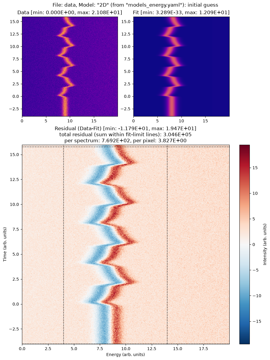
# detail=1 also plots the initial guess; this first evaluation prints the
# subcycle-boundary warning explained above
print("\n=== Model with Multi-Cycle Time Dependence ===")
file.describe_model(model_info='2D', detail=1)
Loading model to describe time-dependence of a model parameter: GLP_01_x0 of IRF_MonoExpNeg_MonoExpPos model

=== Model with Multi-Cycle Time Dependence ===
model name: 2D
function: LinBack from trspecfit.functions.energy
function: GLP from trspecfit.functions.energy
all lmfit.Parameters() [flattened and sorted alphabetically]:
Name                        Value      Min      Max   Stderr     Vary     Expr Brute_Step
GLP_01_A                       12     -inf      inf     None    False     None     None
GLP_01_F                      1.5     -inf      inf     None    False     None     None
GLP_01_m                      0.3     -inf      inf     None    False     None     None
GLP_01_x0                       8        5       15     None     True     None     None
GLP_01_x0_expFun_01_A        -1.5       -5   -0.001     None     True     None     None
GLP_01_x0_expFun_01_t0          0     -inf      inf     None    False     None     None
GLP_01_x0_expFun_01_tau         1     0.05        5     None     True     None     None
GLP_01_x0_expFun_02_A         1.5     -inf      inf     None    False -GLP_01_x0_expFun_01_A     None
GLP_01_x0_expFun_02_t0          0     -inf      inf     None    False     None     None
GLP_01_x0_expFun_02_tau         1     0.05        5     None     True     None     None
GLP_01_x0_gaussCONV_SD        0.1    1e-06        1     None     True     None     None
LinBack_b                       0     -inf      inf     None    False     None     None
LinBack_m                    0.01     -inf      inf     None    False     None     None
LinBack_xStart                  0     -inf      inf     None    False     None     None
LinBack_xStop                  20     -inf      inf     None    False     None     None
<site-packages>/trspecfit/mcp.py:2883: UserWarning: 7 time sample(s) lie within a relative tolerance of 1e-06 of a subcycle boundary (t = 2, 4, 6, 8, 10, ...). Subcycle assignment switches discretely there, so the model prediction for these samples can silently change with the floating-point representation of the time axis (e.g. after saving it to text and reloading). Shift these samples off the boundaries or sample strictly inside subcycles.
  self.normalize_time()  # update the normalization of the time axis
# Perform global 2D fit
file.fit_2d(
    model_name='2D',
    stages=2,
    try_ci=0  # skip confidence intervals: see 12_uncertainty_mcmc
)
Time initialize: 1.8358230590820312e-05 s

Results global minumum fit (method=Nelder):
[[Variables]]
    LinBack_m:                0.08026027 (fixed)
    LinBack_b:                2.000805 (fixed)
    LinBack_xStart:           0 (fixed)
    LinBack_xStop:            20 (fixed)
    GLP_01_A:                 11.90541 (fixed)
    GLP_01_x0:                9.00121749 +/- 0.00124831 (0.01%) (init = 9.000889)
    GLP_01_x0_gaussCONV_SD:   0.14812828 +/- 6.3008e-04 (0.43%) (init = 0.1)
    GLP_01_x0_expFun_01_A:   -1.98182277 +/- 0.00386699 (0.20%) (init = -1.5)
    GLP_01_x0_expFun_01_tau:  0.40615326 +/- 0.00172763 (0.43%) (init = 1)
    GLP_01_x0_expFun_01_t0:   0 (fixed)
    GLP_01_x0_expFun_02_A:    1.98182277 +/- 0.00386699 (0.20%) == '-GLP_01_x0_expFun_01_A'
    GLP_01_x0_expFun_02_tau:  0.80485906 +/- 0.00252634 (0.31%) (init = 1)
    GLP_01_x0_expFun_02_t0:   0 (fixed)
    GLP_01_F:                 1.000414 (fixed)
    GLP_01_m:                 0.1753103 (fixed)
[[Correlations]] (unreported correlations are < 0.100)
    C(GLP_01_x0, GLP_01_x0_expFun_01_tau)               = +0.7038
    C(GLP_01_x0_expFun_01_A, GLP_01_x0_expFun_01_tau)   = +0.5551
    C(GLP_01_x0, GLP_01_x0_expFun_02_tau)               = -0.5118
    C(GLP_01_x0_gaussCONV_SD, GLP_01_x0_expFun_01_A)    = -0.4871
    C(GLP_01_x0_expFun_01_A, GLP_01_x0_expFun_02_tau)   = +0.4726
    C(GLP_01_x0, GLP_01_x0_expFun_01_A)                 = +0.2411
    C(GLP_01_x0_gaussCONV_SD, GLP_01_x0_expFun_01_tau)  = -0.1856
    C(GLP_01_x0_gaussCONV_SD, GLP_01_x0_expFun_02_tau)  = -0.1796
    C(GLP_01_x0_expFun_01_tau, GLP_01_x0_expFun_02_tau) = -0.1027
    C(GLP_01_x0, GLP_01_x0_gaussCONV_SD)                = -0.1002
Time fit (global minimum): 5.486954689025879 s

Results local optimization fit (method=leastsq):
[[Variables]]
    LinBack_m:                0.08026027 (fixed)
    LinBack_b:                2.000805 (fixed)
    LinBack_xStart:           0 (fixed)
    LinBack_xStop:            20 (fixed)
    GLP_01_A:                 11.90541 (fixed)
    GLP_01_x0:                9.00121393 +/- 0.00124873 (0.01%) (init = 9.000889)
    GLP_01_x0_gaussCONV_SD:   0.14812845 +/- 6.2325e-04 (0.42%) (init = 0.1)
    GLP_01_x0_expFun_01_A:   -1.98179539 +/- 0.00385651 (0.19%) (init = -1.5)
    GLP_01_x0_expFun_01_tau:  0.40615328 +/- 0.00173114 (0.43%) (init = 1)
    GLP_01_x0_expFun_01_t0:   0 (fixed)
    GLP_01_x0_expFun_02_A:    1.98179539 +/- 0.00385651 (0.19%) == '-GLP_01_x0_expFun_01_A'
    GLP_01_x0_expFun_02_tau:  0.80487865 +/- 0.00252496 (0.31%) (init = 1)
    GLP_01_x0_expFun_02_t0:   0 (fixed)
    GLP_01_F:                 1.000414 (fixed)
    GLP_01_m:                 0.1753103 (fixed)
[[Correlations]] (unreported correlations are < 0.100)
    C(GLP_01_x0, GLP_01_x0_expFun_01_tau)               = +0.7038
    C(GLP_01_x0_expFun_01_A, GLP_01_x0_expFun_01_tau)   = +0.5555
    C(GLP_01_x0, GLP_01_x0_expFun_02_tau)               = -0.5114
    C(GLP_01_x0_gaussCONV_SD, GLP_01_x0_expFun_01_A)    = -0.4818
    C(GLP_01_x0_expFun_01_A, GLP_01_x0_expFun_02_tau)   = +0.4722
    C(GLP_01_x0, GLP_01_x0_expFun_01_A)                 = +0.2424
    C(GLP_01_x0_gaussCONV_SD, GLP_01_x0_expFun_01_tau)  = -0.1822
    C(GLP_01_x0_gaussCONV_SD, GLP_01_x0_expFun_02_tau)  = -0.1763
    C(GLP_01_x0_expFun_01_tau, GLP_01_x0_expFun_02_tau) = -0.1024
Time fit (local optimization): 0.1912543773651123 s
Time elapsed for 2D model fit: 06.541(ss.ms)
| name | value | standard error | relative error | initial value | min | max | vary | expression |
|---|---|---|---|---|---|---|---|---|
| LinBack_m | 0.08026027 | 0.00000000 | (0.00%) | 0.08026026896038685 | -inf | inf | False | |
| LinBack_b | 2.00080465 | 0.00000000 | (0.00%) | 2.0008046461421696 | -inf | inf | False | |
| LinBack_xStart | 0.00000000 | 0.00000000 | 0.0 | -inf | inf | False | ||
| LinBack_xStop | 20.0000000 | 0.00000000 | (0.00%) | 20.0 | -inf | inf | False | |
| GLP_01_A | 11.9054139 | 0.00000000 | (0.00%) | 11.905413911627253 | -inf | inf | False | |
| GLP_01_x0 | 9.00121393 | 0.00124873 | (0.01%) | 9.000889191102207 | 5.00000000 | 15.0000000 | True | |
| GLP_01_x0_gaussCONV_SD | 0.14812845 | 6.2325e-04 | (0.42%) | 0.1 | 1.0000e-06 | 1.00000000 | True | |
| GLP_01_x0_expFun_01_A | -1.98179539 | 0.00385651 | (0.19%) | -1.5 | -5.00000000 | -1.0000e-03 | True | |
| GLP_01_x0_expFun_01_tau | 0.40615328 | 0.00173114 | (0.43%) | 1.0 | 0.05000000 | 5.00000000 | True | |
| GLP_01_x0_expFun_01_t0 | 0.00000000 | 0.00000000 | 0.0 | -inf | inf | False | ||
| GLP_01_x0_expFun_02_A | 1.98179539 | 0.00385651 | (0.19%) | 1.5 | -inf | inf | False | -GLP_01_x0_expFun_01_A |
| GLP_01_x0_expFun_02_tau | 0.80487865 | 0.00252496 | (0.31%) | 1.0 | 0.05000000 | 5.00000000 | True | |
| GLP_01_x0_expFun_02_t0 | 0.00000000 | 0.00000000 | 0.0 | -inf | inf | False | ||
| GLP_01_F | 1.00041350 | 0.00000000 | (0.00%) | 1.000413500579686 | -inf | inf | False | |
| GLP_01_m | 0.17531026 | 0.00000000 | (0.00%) | 0.17531025870796207 | -inf | inf | False |
5. Inspect the Fit Results#
file.get_parameters(fit_type='2d') returns a pandas.DataFrame with one row per parameter. The subcycle parameters are named by their component, numbered in list order across the dynamics models. GLP_01_x0_expFun_01_* is the expFun of MonoExpNeg (subcycle 1) and GLP_01_x0_expFun_02_* the one of MonoExpPos (subcycle 2); the YAML model names themselves do not appear in parameter names. Note expFun_02_A keeps its expression in the expr column — the mirrored amplitude was never fit independently — while the two tau values are separate free parameters.
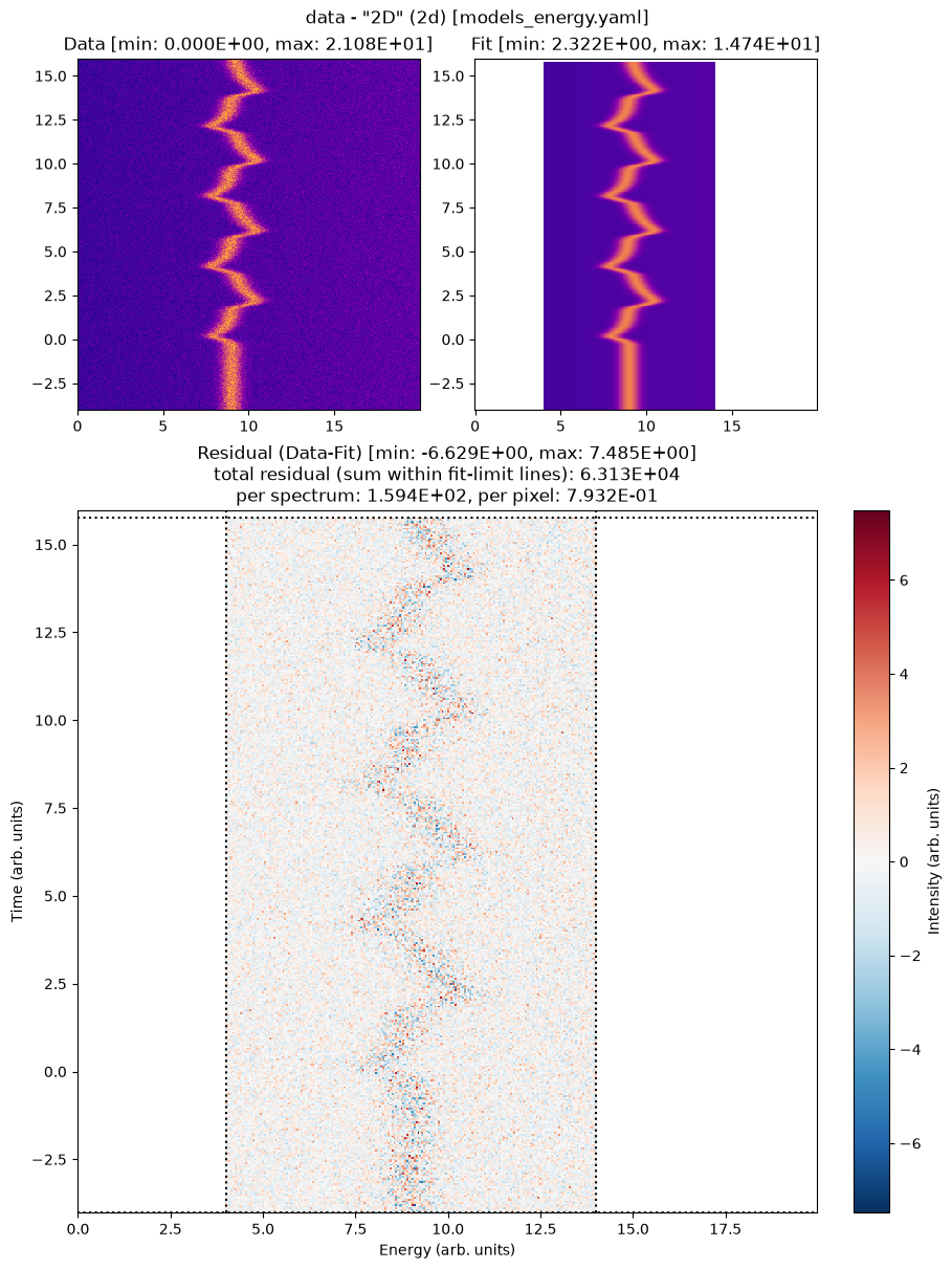
Because the data is synthetic, the results can be compared to the known truth (data/models_*_truth.yaml). The global fit recovers the IRF width (SD ≈ 0.15), the shared shift amplitude (A ≈ −2), and the two distinct relaxation times (tau ≈ 0.4 in subcycle 1 vs ≈ 0.8 in subcycle 2).
One subtlety worth noticing in the fitted curves: with the same amplitude, the visible excursion of subcycle 1 is smaller than subcycle 2’s — its faster relaxation (tau comparable to the IRF width) erodes more of the jump under the convolution. The fit still recovers the true shared amplitude because the IRF is part of the model.
file.get_parameters(fit_type='2d')
| name | value | stderr | init_value | min | max | vary | expr | |
|---|---|---|---|---|---|---|---|---|
| 0 | LinBack_m | 0.080260 | 0.000000 | 0.080260 | -inf | inf | False | NaN |
| 1 | LinBack_b | 2.000805 | 0.000000 | 2.000805 | -inf | inf | False | NaN |
| 2 | LinBack_xStart | 0.000000 | 0.000000 | 0.000000 | -inf | inf | False | NaN |
| 3 | LinBack_xStop | 20.000000 | 0.000000 | 20.000000 | -inf | inf | False | NaN |
| 4 | GLP_01_A | 11.905414 | 0.000000 | 11.905414 | -inf | inf | False | NaN |
| 5 | GLP_01_x0 | 9.001214 | 0.001249 | 9.000889 | 5.000000 | 15.000 | True | NaN |
| 6 | GLP_01_x0_gaussCONV_SD | 0.148128 | 0.000623 | 0.100000 | 0.000001 | 1.000 | True | NaN |
| 7 | GLP_01_x0_expFun_01_A | -1.981795 | 0.003857 | -1.500000 | -5.000000 | -0.001 | True | NaN |
| 8 | GLP_01_x0_expFun_01_tau | 0.406153 | 0.001731 | 1.000000 | 0.050000 | 5.000 | True | NaN |
| 9 | GLP_01_x0_expFun_01_t0 | 0.000000 | 0.000000 | 0.000000 | -inf | inf | False | NaN |
| 10 | GLP_01_x0_expFun_02_A | 1.981795 | 0.003857 | 1.500000 | -inf | inf | False | -GLP_01_x0_expFun_01_A |
| 11 | GLP_01_x0_expFun_02_tau | 0.804879 | 0.002525 | 1.000000 | 0.050000 | 5.000 | True | NaN |
| 12 | GLP_01_x0_expFun_02_t0 | 0.000000 | 0.000000 | 0.000000 | -inf | inf | False | NaN |
| 13 | GLP_01_F | 1.000414 | 0.000000 | 1.000414 | -inf | inf | False | NaN |
| 14 | GLP_01_m | 0.175310 | 0.000000 | 0.175310 | -inf | inf | False | NaN |
Tips for Multi-Cycle Fitting#
Identifying subcycles
Use Slice-by-Slice fits to reveal the repeating pattern and count the distinct phases per period.
Set
frequencyfrom the experiment (pulse timing, modulation frequency) whenever it is known.
Structuring the dynamics_model list
Element 0 applies globally, across all times t. Put the IRF there (
gaussCONV-only model), or a model containing onlynone: {}if there is no global effect.Elements 1+ split each 1/
frequencyperiod equally and run on local clocks that reset at each subcycle start.Link physically shared parameters across subcycle models with expressions (e.g.
"-expFun_01_A"); keep genuinely independent ones (here: the twotau) free.
Strategy
Fit the baseline first; pin line-shape parameters during the 2D fit.
Start with the simple per-subcycle models and add complexity if the residuals demand it.
Next Steps#
Which parameters are truly independent across subcycles? The drive scheme tells you the subcycle structure, but not whether the responses share parameters — fit a fully-linked variant (e.g. shared
tau) against the independent one and compare:10_model_comparisonParameter expressions in depth:
02_dependent_parametersParameters that vary along an auxiliary axis:
04_parameter_profilesUncertainty estimation (MCMC):
12_uncertainty_mcmcSave, load, and export fits:
11_save_load_export
Model files#
The YAML files next to this notebook, as shipped with the example.
models_energy.yaml#
# Use these models to describe the energy-dependent data
# For available functions see: /src/trspecfit/functions/energy.py

# Ground state
# (most parameters should be able to vary)
base:
    LinBack:
      m: [1E-2, True, -1, 1]
      b: [0, True, -5, 5]
      xStart: [0, False]
      xStop: [20, False]
    GLP:
      A: [10, True, 5, 15]
      x0: [8, True, 5, 15]
      F: [1.5, True, 0.75, 2.5]
      m: [0.3, True, 0, 1]

# Slice-by-Slice model fit
# (pinned parameters will be set to "base" Model fit result values)
SbS:
    LinBack:
      m: [1E-2, False]
      b: [0, False]
      xStart: [0, False]
      xStop: [20, False]
    GLP:
      A: [12, False]
      x0: [8, True, 5, 15]
      F: [1.5, False]
      m: [0.3, False]

# 2D model fit
# (pinned parameters will be set to "base" Model fit result values)
2D:
    LinBack:
      m: [1E-2, False]
      b: [0, False]
      xStart: [0, False]
      xStop: [20, False]
    GLP:
      A: [12, False]
      x0: [8, True, 5, 15]
      F: [1.5, False]
      m: [0.3, False]
models_time.yaml#
# Use these models to add multi-cycle time-dependence to a parameter in a 2D model:
# pass a list of model names to add_time_dependence(). Element 0 applies globally
# (all times); elements 1+ alternate as subcycles within each 1/frequency period.
# For available functions see: /src/trspecfit/functions/time.py

# Global element 0: Gaussian instrument response function (IRF).
# Convolves the full time trace, including all subcycles.
# (Use a model containing only `none: {}` here if no global effect is needed.)
IRF:
    gaussCONV:
        SD: [0.1, True, 1.0E-6, 1]

# Subcycle 1: negative exponential shift, relaxing back to 0.
# t0 is on the subcycle's local clock, which resets at each subcycle start.
MonoExpNeg:
    expFun:
        A: [-1.5, True, -5, -1E-3]
        tau: [1, True, 0.05, 5]
        t0: [0, False]

# Subcycle 2: amplitude mirrors subcycle 1 via an expression (no extra free
# parameter), while tau is fit independently — expressions work across
# subcycle models just like across energy components (see 02).
MonoExpPos:
    expFun:
        A: ["-expFun_01_A"]
        tau: [1, True, 0.05, 5]
        t0: [0, False]
project.yaml#
# Project configuration for trspecfit multi_cycle example

# Display settings (general verbosity)
show_output: 1  # 0: silent/API mode, 1: interactive/notebook mode

# Axis labels
e_label: 'Energy (arb. units)' # x -> energy
t_label: 'Time (arb. units)' # y -> time
z_label: 'Intensity (arb. units)' # z -> intensity

# Plot settings
x_dir: 'def'  # def(ault) or rev(erse)
x_type: 'lin'  # lin or log
y_dir: 'def'  # def(ault) or rev(erse)
y_type: 'lin'  # lin or log
z_colormap: 'plasma' # colormap in 2D plots
z_type: 'lin'  # lin or log (2D plots)
dpi_plt: 100 # figure display dpi
dpi_save: 300 # figure save dpi
res_mult: 5 # residual multiplier in figures
The data were generated by data/generate_data.ipynb; its page shows the truth model files.