Comparing Models with FitResults#
This notebook is about model selection — picking the better of two candidates against the same data. The tool for the job is file.compare_models(), which ranks competing models by fit-quality metrics pulled straight from the fit history (no disk I/O). Data is generated inline (§0) so the ground truth stays visible and tunable. The fit-and-compare loop then runs at three fit levels — baseline, slice-by-slice, 2D — each isolating one structural choice, and §4 turns from which model to which configuration of one model:
Section |
Method |
Expected winner |
Challenger |
What it shows |
|---|---|---|---|---|
1 |
|
|
|
Shape matters — Lorentzian tails need the GLP |
2 |
|
|
|
Simplicity matters — the extra free amplitude doesn’t improve the fit when only |
3 |
|
|
|
Instrument response matters — the extra IRF parameter genuinely improves the fit: it captures the smooth onset at |
4 |
|
|
|
Configuration matters — |
Set M_TRUE → 0 and the baseline pair ties; set SD_TRUE → 0 and the 2D pair does.
Fits never write to disk, and this notebook writes no files at all. Persistence, archive inspection, and CSV/PNG export live in the sibling notebook 11_save_load_export, which uses this notebook’s fitted state as its preamble.
from pathlib import Path

import numpy as np
from scipy.ndimage import gaussian_filter1d

import trspecfit
from trspecfit.functions.energy import GLP, LinBack
0. Generate Synthetic Data#
We build the dataset inline so the ground truth is part of the notebook narrative — change a constant and re-run to see how the comparison metrics react.
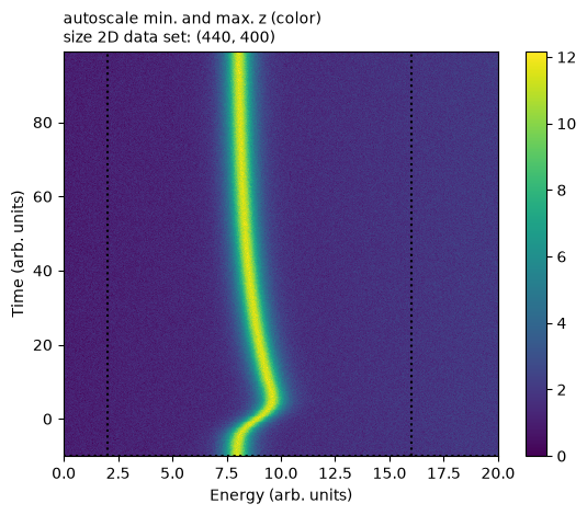
The dynamics follow the classic shift-and-decay pump-probe pattern:
t < 0: peak sits atX0_BASE = 8(ground state).t = 0: the pump shifts the peak position up byDELTA_X = 2— before IRF smearing; the realized maximum is lower (the trajectory printout below shows it).t > 0: peak relaxes back toX0_BASEwith time constantTAU = 30.
The pump and probe pulses have finite duration, so the shift-and-decay is convolved with a Gaussian IRF of width SD_TRUE = 3. That convolution is what the m2d_w_IRF model needs to capture and m2d_wo_IRF cannot.
Peak shape: GLP with
M_TRUE = 0.85(strongly Lorentzian).Background: linear,
m = 0.05,b = 1.0.Noise: Gaussian, σ = 2% of clean-data max.
Array shape:
(n_time, n_energy) = (440, 400).
# --- Ground truth (edit and re-run to see the comparison react) ----------
M_TRUE = 0.85    # GLP mixing: 0 = pure Gaussian, 1 = pure Lorentzian
A_TRUE = 10.0
F_TRUE = 1.0
X0_BASE = 8.0    # peak position at t < 0 and t -> ∞
DELTA_X = 2.0    # shift amplitude at t = 0 (matches expFun A)
TAU = 30.0       # decay time back to X0_BASE
SD_TRUE = 3.0    # instrument-response Gaussian σ (time units)
LIN_M = 0.05
LIN_B = 1.0
NOISE_REL = 0.02

# --- Axes -----------------------------------------------------------------
energy = np.linspace(0.0, 20.0, 400)
time = np.linspace(-10.0, 99.0, 440)

# --- Time-dependent peak position: shift-and-decay ⊗ IRF (see md above) ---
shift_sharp = np.where(time < 0, 0.0, DELTA_X * np.exp(-time / TAU))
dt = float(time[1] - time[0])
shift_smoothed = gaussian_filter1d(shift_sharp, sigma=SD_TRUE / dt, mode="nearest")
x0_t = X0_BASE + shift_smoothed

# --- Build the clean 2D model: GLP shifted in time + linear background ----
back = LinBack(energy, LIN_M, LIN_B, energy.min(), energy.max(), spectrum=None)
clean = np.stack(
    [GLP(energy, A_TRUE, x0, F_TRUE, M_TRUE) + back for x0 in x0_t]
)

# --- Add noise; NOISE_SIGMA goes into file.set_sigma below ----------------
NOISE_SIGMA = NOISE_REL * clean.max()
rng = np.random.default_rng(42)
data = clean + rng.normal(scale=NOISE_SIGMA, size=clean.shape)

# --- Wire into a Project / File ------------------------------------------
project = trspecfit.Project(path=Path.cwd(), name="model_comparison")
file = trspecfit.File(
    parent_project=project,
    path="synthetic",
    data=data,
    energy=energy,
    time=time,
)
# Register the per-pixel σ once on the File; every later fit minimizes
# (data − model)/σ and records σ-calibrated metrics in its saved slot
# (full semantics: see Tips).
file.set_sigma(NOISE_SIGMA)

print(f"File name:        {file.name}")
print(f"Data shape:       {file.data.shape}")
print(f"True GLP m:       {M_TRUE}   (base_Gauss → wrong line shape)")
print(f"True IRF σ:       {SD_TRUE}   (m2d_wo_IRF → sharp turn-on)")
print(f"file.sigma_data:  {file.sigma_data:.4f}   "
      f"(noise_type={file.noise_type!r})")
print(f"x0 trajectory:    starts at {x0_t[0]:.2f}, peaks at {x0_t.max():.2f}, "
      f"ends at {x0_t[-1]:.2f}")
File name:        synthetic
Data shape:       (440, 400)
True GLP m:       0.85   (base_Gauss → wrong line shape)
True IRF σ:       3.0   (m2d_wo_IRF → sharp turn-on)
file.sigma_data:  0.2296   (noise_type='gaussian')
x0 trajectory:    starts at 8.00, peaks at 9.60, ends at 8.08
1. Baseline#
1.1 Define Data and Fit Limits#
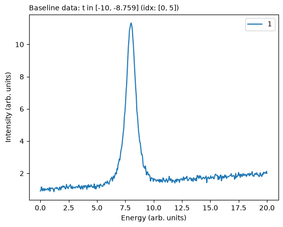
Same limits for both models, so both fit the same points and their metrics are comparable.
The baseline window must end early enough that the IRF-smeared onset can’t leak backwards into it; a practical rule is about 3·SD_TRUE before t0. Here 3·SD_TRUE = 9 and the time axis starts at −10, so only the first few slices qualify. The cleaner fix is more pre-t0 data (extend the time axis when generating or measuring), but this notebook deliberately keeps the short pre-t0 range and a tight window to keep the dataset small.
# time_limits spans the full axis; energy_limits trims the empty wings
file.set_fit_limits(energy_limits=[2, 16], time_limits=[time[0], time[-1]])
# time_type="ind" reads the window as slice indices, not time-axis units
file.define_baseline(time_start=0, time_stop=5, time_type="ind")
1.2 Fit Two Baseline Models#
Each fit_baseline call appends its result to the project’s fit history, so even though file.model_base is overwritten by the second fit, both results stay available for the comparison.
Fit order still matters, because of seeding: subsequent SbS and 2D fits pin their non-varying parameters from file.model_base.result — the most recent baseline. We fit base_Gauss first and base_GLP last so the correct GLP shape is what gets pinned downstream.
# base_Gauss first: pure Gaussian peak.
# stages=2 fits twice: a simplex pass, then leastsq refinement.
# try_ci=0 skips confidence intervals: see 12_uncertainty_mcmc
file.load_model(model_yaml="models_energy.yaml", model_info="base_Gauss")
file.fit_baseline(model_name="base_Gauss", stages=2, try_ci=0)

# base_GLP last: leaves model_base.result holding the correct GLP shape
file.load_model(model_yaml="models_energy.yaml", model_info="base_GLP")
file.fit_baseline(model_name="base_GLP", stages=2, try_ci=0)

print(f"\nFits recorded: {len(project.results.find(file=file.name))}")
print("Models seen:", project.results.models(file=file.name))
Loading model to describe energy- (and time-)dependent data: base_Gauss

Time initialize: 6.079673767089844e-05 s

Results global minumum fit (method=Nelder):
[[Variables]]
    LinBack_m:       0.04590084 +/- 0.00139492 (3.04%) (init = 0.01)
    LinBack_b:       1.09841511 +/- 0.01431742 (1.30%) (init = 0)
    LinBack_xStart:  0 (fixed)
    LinBack_xStop:   20 (fixed)
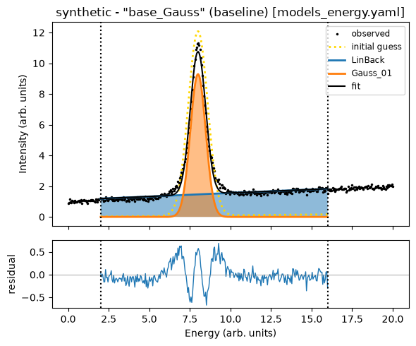
    Gauss_01_A:      9.29353534 +/- 0.02950836 (0.32%) (init = 12)
    Gauss_01_x0:     8.00189778 +/- 0.00164985 (0.02%) (init = 8)
    Gauss_01_SD:     0.47164916 +/- 0.00194212 (0.41%) (init = 0.6)
[[Correlations]] (unreported correlations are < 0.100)
    C(LinBack_m, LinBack_b)    = -0.9000
    C(Gauss_01_A, Gauss_01_SD) = -0.5547
    C(LinBack_b, Gauss_01_SD)  = -0.1995
Time fit (global minimum): 0.05255436897277832 s

Results local optimization fit (method=leastsq):
[[Variables]]
    LinBack_m:       0.04592025 +/- 0.00139389 (3.04%) (init = 0.01)
    LinBack_b:       1.09820395 +/- 0.01425312 (1.30%) (init = 0)
    LinBack_xStart:  0 (fixed)
    LinBack_xStop:   20 (fixed)
    Gauss_01_A:      9.29364278 +/- 0.02847035 (0.31%) (init = 12)
    Gauss_01_x0:     8.00192215 +/- 0.00164982 (0.02%) (init = 8)
    Gauss_01_SD:     0.47164718 +/- 0.00171010 (0.36%) (init = 0.6)
[[Correlations]] (unreported correlations are < 0.100)
    C(LinBack_m, LinBack_b)    = -0.9011
    C(Gauss_01_A, Gauss_01_SD) = -0.5062
    C(LinBack_b, Gauss_01_SD)  = -0.1764
    C(LinBack_b, Gauss_01_A)   = -0.1044
Time fit (local optimization): 0.004006147384643555 s
Time elapsed for baseline fit: 00.333(ss.ms)
Loading model to describe energy- (and time-)dependent data: base_GLP

Time initialize: 1.6450881958007812e-05 s

Results global minumum fit (method=Nelder):
[[Variables]]
    LinBack_m:       0.05034827 +/- 0.00140792 (2.80%) (init = 0.01)
    LinBack_b:       0.98589315 +/- 0.01510261 (1.53%) (init = 0)
    LinBack_xStart:  0 (fixed)
    LinBack_xStop:   20 (fixed)
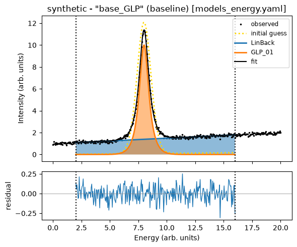
    GLP_01_A:        10.0120833 +/- 0.03707021 (0.37%) (init = 12)
    GLP_01_x0:       8.00127670 +/- 0.00159286 (0.02%) (init = 8)
    GLP_01_F:        0.99715681 +/- 0.00640625 (0.64%) (init = 1.5)
    GLP_01_m:        0.85859477 +/- 0.00851419 (0.99%) (init = 0.3)
[[Correlations]] (unreported correlations are < 0.100)
    C(LinBack_m, LinBack_b) = -0.8883
    C(GLP_01_F, GLP_01_m)   = -0.7127
    C(GLP_01_A, GLP_01_F)   = -0.7038
    C(GLP_01_A, GLP_01_m)   = +0.4909
    C(LinBack_b, GLP_01_m)  = -0.2739
    C(LinBack_b, GLP_01_A)  = -0.1815
    C(LinBack_m, GLP_01_m)  = +0.1158
Time fit (global minimum): 0.12050533294677734 s

Results local optimization fit (method=leastsq):
[[Variables]]
    LinBack_m:       0.05034939 +/- 0.00140799 (2.80%) (init = 0.01)
    LinBack_b:       0.98587835 +/- 0.01510839 (1.53%) (init = 0)
    LinBack_xStart:  0 (fixed)
    LinBack_xStop:   20 (fixed)
    GLP_01_A:        10.0121416 +/- 0.03720326 (0.37%) (init = 12)
    GLP_01_x0:       8.00127749 +/- 0.00159190 (0.02%) (init = 8)
    GLP_01_F:        0.99714273 +/- 0.00645353 (0.65%) (init = 1.5)
    GLP_01_m:        0.85861863 +/- 0.00858656 (1.00%) (init = 0.3)
[[Correlations]] (unreported correlations are < 0.100)
    C(LinBack_m, LinBack_b) = -0.8882
    C(GLP_01_F, GLP_01_m)   = -0.7167
    C(GLP_01_A, GLP_01_F)   = -0.7063
    C(GLP_01_A, GLP_01_m)   = +0.4957
    C(LinBack_b, GLP_01_m)  = -0.2749
    C(LinBack_b, GLP_01_A)  = -0.1828
    C(LinBack_m, GLP_01_m)  = +0.1161
Time fit (local optimization): 0.0029196739196777344 s
Time elapsed for baseline fit: 00.387(ss.ms)

Fits recorded: 2
Models seen: ['base_Gauss', 'base_GLP']
| name | value | standard error | relative error | initial value | min | max | vary |
|---|---|---|---|---|---|---|---|
| LinBack_m | 0.04592025 | 0.00139389 | (3.04%) | 0.01 | -1.00000000 | 1.00000000 | True |
| LinBack_b | 1.09820395 | 0.01425312 | (1.30%) | 0.0 | -5.00000000 | 5.00000000 | True |
| LinBack_xStart | 0.00000000 | 0.00000000 | 0.0 | -inf | inf | False | |
| LinBack_xStop | 20.0000000 | 0.00000000 | (0.00%) | 20.0 | -inf | inf | False |
| Gauss_01_A | 9.29364278 | 0.02847035 | (0.31%) | 12.0 | 5.00000000 | 15.0000000 | True |
| Gauss_01_x0 | 8.00192215 | 0.00164982 | (0.02%) | 8.0 | 5.00000000 | 15.0000000 | True |
| Gauss_01_SD | 0.47164718 | 0.00171010 | (0.36%) | 0.6 | 0.20000000 | 2.50000000 | True |
| name | value | standard error | relative error | initial value | min | max | vary |
|---|---|---|---|---|---|---|---|
| LinBack_m | 0.05034939 | 0.00140799 | (2.80%) | 0.01 | -1.00000000 | 1.00000000 | True |
| LinBack_b | 0.98587835 | 0.01510839 | (1.53%) | 0.0 | -5.00000000 | 5.00000000 | True |
| LinBack_xStart | 0.00000000 | 0.00000000 | 0.0 | -inf | inf | False | |
| LinBack_xStop | 20.0000000 | 0.00000000 | (0.00%) | 20.0 | -inf | inf | False |
| GLP_01_A | 10.0121416 | 0.03720326 | (0.37%) | 12.0 | 5.00000000 | 15.0000000 | True |
| GLP_01_x0 | 8.00127749 | 0.00159190 | (0.02%) | 8.0 | 5.00000000 | 15.0000000 | True |
| GLP_01_F | 0.99714273 | 0.00645353 | (0.65%) | 1.5 | 0.75000000 | 2.50000000 | True |
| GLP_01_m | 0.85861863 | 0.00858656 | (1.00%) | 0.3 | 0.00000000 | 1.00000000 | True |
1.3 Compare the Baseline Fits#
file.compare_models(...) returns a pandas.DataFrame with one row per fit slot, identified by its short handle. The leading columns are file / model / fit_type and selection_json, the fit window as index ranges into the time and energy axes (base_t_ind, e_lim), followed by one column per requested metric.
Column meanings
chi2_red_raw = Σ(observed − fit)² / (N − p)is the unweighted diagnostic in units of (data units)².chi2_red = chi2_red_raw / sigma_eff²is the σ-calibrated value — present only when a sigma was set on the file at fit time (we did that in §0 viafile.set_sigma(NOISE_SIGMA)). This is the canonical “≈ 1 for a good fit” unitless benchmark.sigma_effis the per-row σ that was actually applied. Baseline rows averageN_avgslices, so theirs isNOISE_SIGMA / √N_avg(N_avgfrom the slot’sbase_t_ind); SbS, 2D, and spectrum rows useNOISE_SIGMAverbatim.
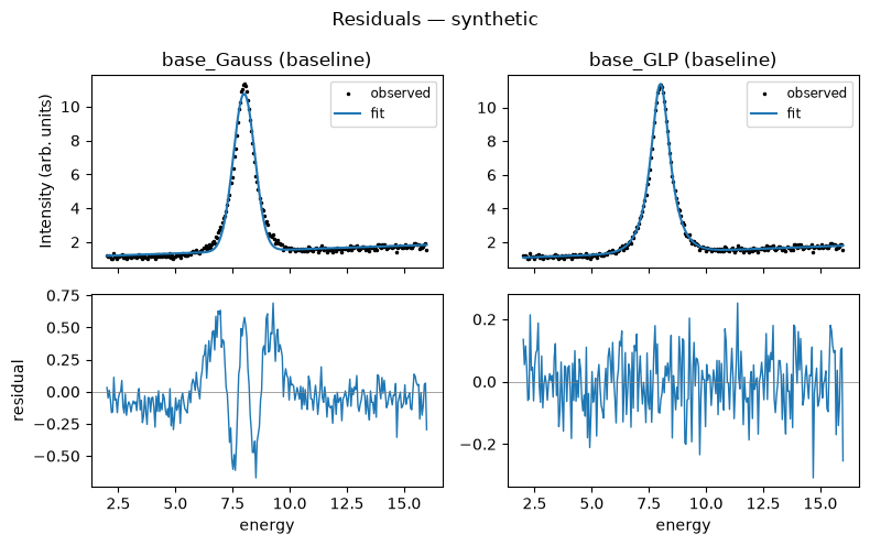
base_Gauss will land well above 1.0 since a pure Gaussian can’t represent the Lorentzian tails.
# one row per baseline slot; chi2_red ≈ 1 marks the line shape that matches
file.compare_models(fit_type="baseline")
| file | model | fit_type | handle | selection_json | chi2_red_raw | sigma_eff | chi2_red | r2 | aic | bic | |
|---|---|---|---|---|---|---|---|---|---|---|---|
| 0 | synthetic | base_Gauss | baseline | 66abe7af | {"base_t_ind": [0, 6], "e_lim": [40, 320]} | 0.051192 | 0.093723 | 5.827871 | 0.988938 | 1612.664494 | 1630.838442 |
| 1 | synthetic | base_GLP | baseline | 0e4fa26e | {"base_t_ind": [0, 6], "e_lim": [40, 320]} | 0.008824 | 0.093723 | 1.004512 | 0.998100 | 287.236404 | 309.045141 |
FitResults.plot_residuals is a quick visual cross-check, not a publication figure: one column per model on the real energy axis, observed and fit on top, the residual below, each residual panel on its own scale (the 2D variant in §3.2 shares one color scale). It shows what the χ² column summarises: base_Gauss leaves a structured, symmetric misfit around the peak several times the noise, the signature of a Gaussian forced onto Lorentzian tails, while the base_GLP residual is noise-like. Build your own from slot.observed / slot.fit for anything fancier.
# residual cross-check of the two baseline fits
project.results.plot_residuals(
    file=file,
    models=["base_GLP", "base_Gauss"],
    fit_type="baseline",
);
2. Slice-by-Slice#
2.1 Fit Two Slice-by-Slice Models#
Pinned (non-varying) parameters seed from file.model_base.result — base_GLP at this point, since we fit it last in §1.2.
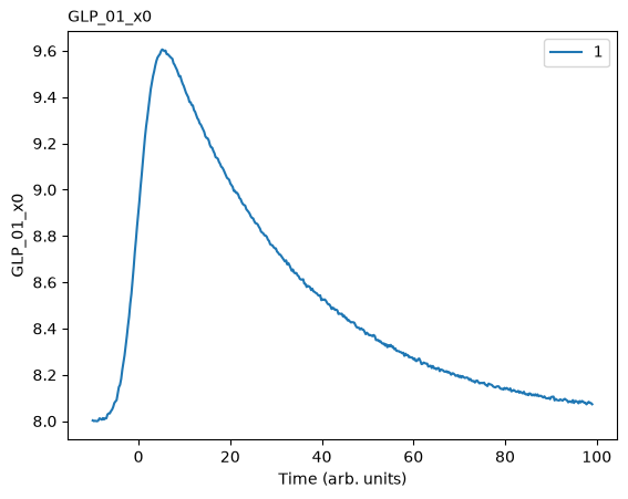
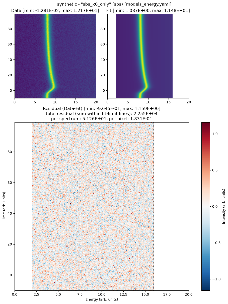
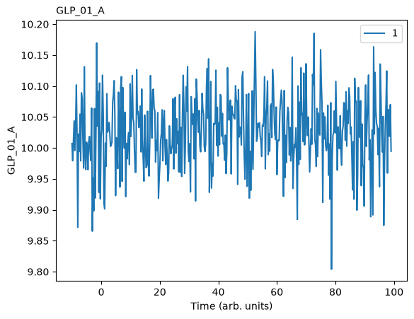
sbs_x0_only: onlyx0floats per slice (truth-like — the simulation moves onlyx0).sbs_x0_A:x0and peak amplitudeAboth float per slice (extra free parameter).
file.load_model(model_yaml="models_energy.yaml", model_info="sbs_x0_only")
file.fit_slice_by_slice(model_name="sbs_x0_only", try_ci=0)

file.load_model(model_yaml="models_energy.yaml", model_info="sbs_x0_A")
file.fit_slice_by_slice(model_name="sbs_x0_A", try_ci=0)

print("\nSbS slots:")
for slot in project.results.find(file=file.name, fit_type="sbs"):
    # count slices via any per-slice metric column
    n_slices = len(slot.metrics["chi2_red_raw"])
    print(f"  {slot.model_name}: {n_slices} slices")
Loading model to describe energy- (and time-)dependent data: sbs_x0_only
Time elapsed for Slice-by-Slice fit: 06.349(ss.ms)
Loading model to describe energy- (and time-)dependent data: sbs_x0_A
Time elapsed for Slice-by-Slice fit: 06.451(ss.ms)

SbS slots:
  sbs_x0_only: 440 slices
  sbs_x0_A: 440 slices
SbS fit (15 workers): 100%|██████████| 440/440 [00:04<00:00, 97.42it/s]
SbS fit (15 workers): 100%|██████████| 440/440 [00:04<00:00, 96.59it/s]
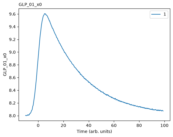
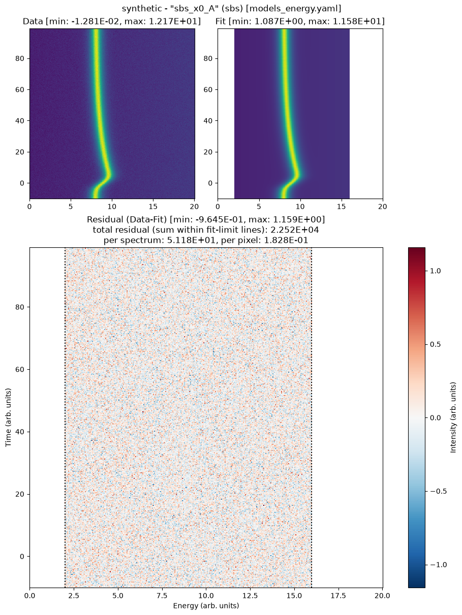
2.2 SbS Comparison — Aggregation Modes#
Per-slice metrics need to be collapsed to compare SbS slots in a single row. sbs_aggregation controls how:
Mode |
What it computes |
When to use it |
|---|---|---|
|
|
robust one-row summary per model |
|
|
like median, but sensitive to outlier slices |
|
|
read the whole batch as one composite fit |
|
no aggregation — one row per slice, plus a |
per-slice questions (see below) |
Two footnotes:
In
"sum"mode ther2column is meaningless — per-slice r² values near 1 just add up to ≈ N_slices (no per-slice SST is stored to compute a true aggregate r²). Ignore it there."long"rows come out slice-major — both models at slice 0, then slice 1, … — so ahead()lines the competing models up at the same slice.sigma_effis a per-fit scalar, broadcast to every slice row.
# Default (median) aggregation — one row per slot
file.compare_models(fit_type="sbs")
| file | model | fit_type | handle | selection_json | chi2_red_raw | sigma_eff | chi2_red | r2 | aic | bic | |
|---|---|---|---|---|---|---|---|---|---|---|---|
| 0 | synthetic | sbs_x0_only | sbs | 1f338da7 | {"e_lim": [40, 320], "t_lim": null} | 0.052886 | 0.229574 | 1.003453 | 0.988608 | 281.963435 | 285.598224 |
| 1 | synthetic | sbs_x0_A | sbs | f9534f93 | {"e_lim": [40, 320], "t_lim": null} | 0.052840 | 0.229574 | 1.002587 | 0.988650 | 282.719157 | 289.988736 |
# Sum aggregation (sum_df is reused by Q2 below): additive metrics total
# across slices; the reduced-χ² columns use Σnumerator / ΣDoF (table above).
sum_df = file.compare_models(fit_type="sbs", sbs_aggregation="sum")
sum_df
| file | model | fit_type | handle | selection_json | chi2_red_raw | sigma_eff | chi2_red | r2 | aic | bic | |
|---|---|---|---|---|---|---|---|---|---|---|---|
| 0 | synthetic | sbs_x0_only | sbs | 1f338da7 | {"e_lim": [40, 320], "t_lim": null} | 0.052946 | 0.229574 | 1.004596 | 434.990772 | 124204.257287 | 125803.564713 |
| 1 | synthetic | sbs_x0_A | sbs | f9534f93 | {"e_lim": [40, 320], "t_lim": null} | 0.052947 | 0.229574 | 1.004608 | 435.008632 | 124643.596071 | 127842.210922 |
# Long form, slice-major: head(6) is the first three slices, both models
# side by side.
long_df = file.compare_models(fit_type="sbs", sbs_aggregation="long")
print(f"long-form rows: {len(long_df)}")
long_df.head(6)
long-form rows: 880
| file | model | fit_type | handle | selection_json | slice_index | chi2_red_raw | sigma_eff | chi2_red | r2 | aic | bic | |
|---|---|---|---|---|---|---|---|---|---|---|---|---|
| 0 | synthetic | sbs_x0_only | sbs | 1f338da7 | {"e_lim": [40, 320], "t_lim": null} | 0 | 0.047670 | 0.229574 | 0.904483 | 0.989630 | 254.350708 | 257.985497 |
| 1 | synthetic | sbs_x0_A | sbs | f9534f93 | {"e_lim": [40, 320], "t_lim": null} | 0 | 0.047840 | 0.229574 | 0.907706 | 0.989630 | 256.342380 | 263.611959 |
| 2 | synthetic | sbs_x0_only | sbs | 1f338da7 | {"e_lim": [40, 320], "t_lim": null} | 1 | 0.054876 | 0.229574 | 1.041213 | 0.988017 | 292.498431 | 296.133221 |
| 3 | synthetic | sbs_x0_A | sbs | f9534f93 | {"e_lim": [40, 320], "t_lim": null} | 1 | 0.055017 | 0.229574 | 1.043877 | 0.988029 | 294.197827 | 301.467406 |
| 4 | synthetic | sbs_x0_only | sbs | 1f338da7 | {"e_lim": [40, 320], "t_lim": null} | 2 | 0.049049 | 0.229574 | 0.930657 | 0.989294 | 261.653396 | 265.288186 |
| 5 | synthetic | sbs_x0_A | sbs | f9534f93 | {"e_lim": [40, 320], "t_lim": null} | 2 | 0.049226 | 0.229574 | 0.934005 | 0.989294 | 263.653396 | 270.922976 |
# A quick pivot: chi2_red per slice for each model, side by side.
wide = long_df.pivot(index="slice_index", columns="model", values="chi2_red")
wide.describe()
| model | sbs_x0_A | sbs_x0_only |
|---|---|---|
| count | 440.000000 | 440.000000 |
| mean | 1.004608 | 1.004596 |
| std | 0.081439 | 0.080957 |
| min | 0.681116 | 0.687799 |
| 25% | 0.944924 | 0.945088 |
| 50% | 1.002587 | 1.003453 |
| 75% | 1.055701 | 1.056632 |
| max | 1.276110 | 1.273818 |
The two columns are indistinguishable: per slice, the extra free amplitude buys nothing in chi2_red. That is the case for the simpler model, and Q2 below makes it formal with the summed AIC/BIC.
The aggregation modes above exist to answer two different questions:
“Which model fits slice 3 best?” — a per-member question. Use long form and filter to that one slice. SbS fits each row as an independent 1D spectrum, so this is the natural tool for a batch of spectra that vary in any parameter (fluence, pressure, position, …), not just a time series — pick whichever slice you care about.
“Which model fits best across the board?” — an aggregate question. Collapse the per-slice metrics to one row per model (
"sum"here reads the batch as one composite fit) and take the lowest AIC/BIC.
# Q1 — best model for slice 3: filter long form to that one slice and compare
# the models head-to-head. Lowest AIC wins; chi2_red shows how close each
# sits to the noise floor at this single spectrum.
cols = ["model", "slice_index", "chi2_red", "aic", "bic"]
long_df[long_df["slice_index"] == 3].sort_values("aic")[cols]
| model | slice_index | chi2_red | aic | bic | |
|---|---|---|---|---|---|
| 6 | sbs_x0_only | 3 | 1.132424 | 317.946355 | 321.581145 |
| 7 | sbs_x0_A | 3 | 1.135476 | 319.662226 | 326.931805 |
# Q2 — best model across the whole batch: sort the sum-aggregated table
# from above; lowest total AIC/BIC wins.
sum_df.sort_values("aic")[["model", "chi2_red", "aic", "bic"]]
| model | chi2_red | aic | bic | |
|---|---|---|---|---|
| 0 | sbs_x0_only | 1.004596 | 124204.257287 | 125803.564713 |
| 1 | sbs_x0_A | 1.004608 | 124643.596071 | 127842.210922 |
3. 2D Fit#
3.1 Fit 2D Models#
The truth x0(t) is a shift-and-decay convolved with a Gaussian IRF. We fit two competing time-dependence models on the same energy backbone:
m2d_w_IRF+MonoExpPosIRF— shift-and-decay convolved withgaussCONV. Matches truth structurally. One extra free parameter (gaussCONV SD).m2d_wo_IRF+MonoExpPos— bare shift-and-decay, no IRF. Sharp turn-on att = 0; cannot reproduce the smooth onset.
# m2d_w_IRF: gaussCONV ⊗ expFun — matches truth
file.load_model(model_yaml="models_energy.yaml", model_info="m2d_w_IRF")
file.add_time_dependence(
    target_model="m2d_w_IRF",
    target_parameter="GLP_01_x0",
    dynamics_yaml="models_time.yaml",
    dynamics_model="MonoExpPosIRF",
)
file.fit_2d(model_name="m2d_w_IRF", stages=2, try_ci=0)
Loading model to describe energy- (and time-)dependent data: m2d_w_IRF
Loading model to describe time-dependence of a model parameter: GLP_01_x0 of MonoExpPosIRF model

Time initialize: 1.3113021850585938e-05 s

Results global minumum fit (method=Nelder):
[[Variables]]
    LinBack_m:                0.05034939 (fixed)
    LinBack_b:                0.9858783 (fixed)
    LinBack_xStart:           0 (fixed)
    LinBack_xStop:            20 (fixed)
    GLP_01_A:                 10.01214 (fixed)
    GLP_01_x0:                7.99943548 +/- 4.6019e-04 (0.01%) (init = 8.001277)
    GLP_01_x0_gaussCONV_SD:   3.01302778 +/- 0.00509283 (0.17%) (init = 3)
    GLP_01_x0_expFun_01_A:    2.00239755 +/- 9.3694e-04 (0.05%) (init = 2)
    GLP_01_x0_expFun_01_tau:  29.9715964 +/- 0.02632894 (0.09%) (init = 30)
    GLP_01_x0_expFun_01_t0:   0 (fixed)
    GLP_01_F:                 0.9971427 (fixed)
    GLP_01_m:                 0.8586186 (fixed)
[[Correlations]] (unreported correlations are < 0.100)
    C(GLP_01_x0, GLP_01_x0_expFun_01_tau)             = -0.7527
    C(GLP_01_x0_gaussCONV_SD, GLP_01_x0_expFun_01_A)  = +0.4543
    C(GLP_01_x0, GLP_01_x0_expFun_01_A)               = -0.3219
    C(GLP_01_x0_expFun_01_A, GLP_01_x0_expFun_01_tau) = -0.2431
    C(GLP_01_x0, GLP_01_x0_gaussCONV_SD)              = -0.2059
Time fit (global minimum): 0.8385233879089355 s

Results local optimization fit (method=leastsq):
[[Variables]]
    LinBack_m:                0.05034939 (fixed)
    LinBack_b:                0.9858783 (fixed)
    LinBack_xStart:           0 (fixed)
    LinBack_xStop:            20 (fixed)
    GLP_01_A:                 10.01214 (fixed)
    GLP_01_x0:                7.99943381 +/- 4.6012e-04 (0.01%) (init = 8.001277)
    GLP_01_x0_gaussCONV_SD:   3.01303066 +/- 0.00509034 (0.17%) (init = 3)
    GLP_01_x0_expFun_01_A:    2.00240123 +/- 9.3749e-04 (0.05%) (init = 2)
    GLP_01_x0_expFun_01_tau:  29.9716052 +/- 0.02632576 (0.09%) (init = 30)
    GLP_01_x0_expFun_01_t0:   0 (fixed)
    GLP_01_F:                 0.9971427 (fixed)
    GLP_01_m:                 0.8586186 (fixed)
[[Correlations]] (unreported correlations are < 0.100)
    C(GLP_01_x0, GLP_01_x0_expFun_01_tau)             = -0.7523
    C(GLP_01_x0_gaussCONV_SD, GLP_01_x0_expFun_01_A)  = +0.4537
    C(GLP_01_x0, GLP_01_x0_expFun_01_A)               = -0.3222
    C(GLP_01_x0_expFun_01_A, GLP_01_x0_expFun_01_tau) = -0.2434
    C(GLP_01_x0, GLP_01_x0_gaussCONV_SD)              = -0.2075
Time fit (local optimization): 0.05999422073364258 s
Time elapsed for 2D model fit: 01.762(ss.ms)
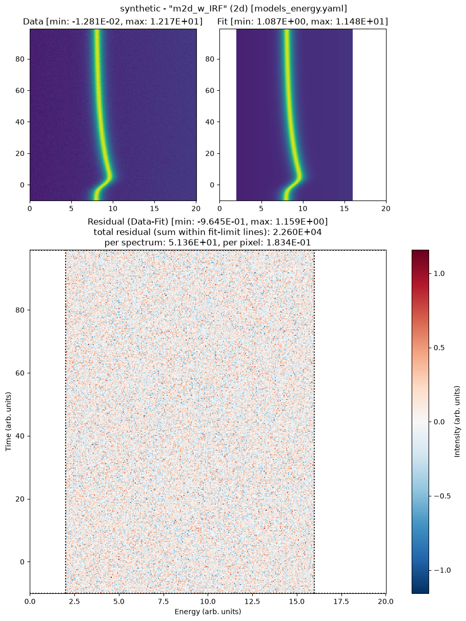
| name | value | standard error | relative error | initial value | min | max | vary |
|---|---|---|---|---|---|---|---|
| LinBack_m | 0.05034939 | 0.00000000 | (0.00%) | 0.05034939429426233 | -inf | inf | False |
| LinBack_b | 0.98587835 | 0.00000000 | (0.00%) | 0.9858783483405809 | -inf | inf | False |
| LinBack_xStart | 0.00000000 | 0.00000000 | 0.0 | -inf | inf | False | |
| LinBack_xStop | 20.0000000 | 0.00000000 | (0.00%) | 20.0 | -inf | inf | False |
| GLP_01_A | 10.0121416 | 0.00000000 | (0.00%) | 10.012141588731303 | -inf | inf | False |
| GLP_01_x0 | 7.99943381 | 4.6012e-04 | (0.01%) | 8.001277485561658 | 5.00000000 | 15.0000000 | True |
| GLP_01_x0_gaussCONV_SD | 3.01303066 | 0.00509034 | (0.17%) | 3.0 | 1.0000e-06 | 10.0000000 | True |
| GLP_01_x0_expFun_01_A | 2.00240123 | 9.3749e-04 | (0.05%) | 2.0 | 0.00000000 | 10.0000000 | True |
| GLP_01_x0_expFun_01_tau | 29.9716052 | 0.02632576 | (0.09%) | 30.0 | 1.00000000 | 100.000000 | True |
| GLP_01_x0_expFun_01_t0 | 0.00000000 | 0.00000000 | 0.0 | -inf | inf | False | |
| GLP_01_F | 0.99714273 | 0.00000000 | (0.00%) | 0.9971427278389471 | -inf | inf | False |
| GLP_01_m | 0.85861863 | 0.00000000 | (0.00%) | 0.8586186275153562 | -inf | inf | False |
# m2d_wo_IRF: sharp expFun turn-on — structurally wrong at t ≈ 0
file.load_model(model_yaml="models_energy.yaml", model_info="m2d_wo_IRF")
file.add_time_dependence(
    target_model="m2d_wo_IRF",
    target_parameter="GLP_01_x0",
    dynamics_yaml="models_time.yaml",
    dynamics_model="MonoExpPos",
)
file.fit_2d(model_name="m2d_wo_IRF", stages=2, try_ci=0)
Loading model to describe energy- (and time-)dependent data: m2d_wo_IRF
Loading model to describe time-dependence of a model parameter: GLP_01_x0 of MonoExpPos model

Time initialize: 1.1682510375976562e-05 s

Results global minumum fit (method=Nelder):
[[Variables]]
    LinBack_m:                0.05034939 (fixed)
    LinBack_b:                0.9858783 (fixed)
    LinBack_xStart:           0 (fixed)
    LinBack_xStop:            20 (fixed)
    GLP_01_A:                 10.01214 (fixed)
    GLP_01_x0:                8.03909907 +/- 4.5285e-04 (0.01%) (init = 8.001277)
    GLP_01_x0_expFun_01_A:    1.77159970 +/- 8.2786e-04 (0.05%) (init = 2)
    GLP_01_x0_expFun_01_tau:  31.4401908 +/- 0.02939120 (0.09%) (init = 30)
    GLP_01_x0_expFun_01_t0:   0 (fixed)
    GLP_01_F:                 0.9971427 (fixed)
    GLP_01_m:                 0.8586186 (fixed)
[[Correlations]] (unreported correlations are < 0.100)
    C(GLP_01_x0, GLP_01_x0_expFun_01_tau)             = -0.7774
    C(GLP_01_x0_expFun_01_A, GLP_01_x0_expFun_01_tau) = -0.2663
    C(GLP_01_x0, GLP_01_x0_expFun_01_A)               = -0.2426
Time fit (global minimum): 0.6444694995880127 s

Results local optimization fit (method=leastsq):
[[Variables]]
    LinBack_m:                0.05034939 (fixed)
    LinBack_b:                0.9858783 (fixed)
    LinBack_xStart:           0 (fixed)
    LinBack_xStop:            20 (fixed)
    GLP_01_A:                 10.01214 (fixed)
    GLP_01_x0:                8.03909907 +/- 4.5245e-04 (0.01%) (init = 8.001277)
    GLP_01_x0_expFun_01_A:    1.77159970 +/- 7.2952e-04 (0.04%) (init = 2)
    GLP_01_x0_expFun_01_tau:  31.4401908 +/- 0.03028088 (0.10%) (init = 30)
    GLP_01_x0_expFun_01_t0:   0 (fixed)
    GLP_01_F:                 0.9971427 (fixed)
    GLP_01_m:                 0.8586186 (fixed)
[[Correlations]] (unreported correlations are < 0.100)
    C(GLP_01_x0, GLP_01_x0_expFun_01_tau)             = -0.8021
    C(GLP_01_x0, GLP_01_x0_expFun_01_A)               = -0.2610
    C(GLP_01_x0_expFun_01_A, GLP_01_x0_expFun_01_tau) = -0.2043
Time fit (local optimization): 0.03781628608703613 s
Time elapsed for 2D model fit: 01.524(ss.ms)
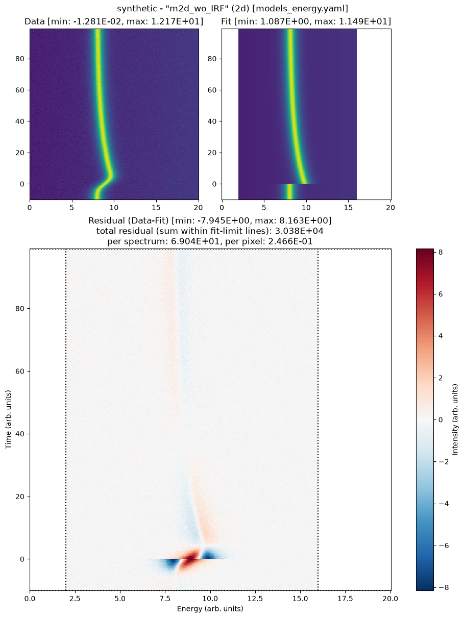
| name | value | standard error | relative error | initial value | min | max | vary |
|---|---|---|---|---|---|---|---|
| LinBack_m | 0.05034939 | 0.00000000 | (0.00%) | 0.05034939429426233 | -inf | inf | False |
| LinBack_b | 0.98587835 | 0.00000000 | (0.00%) | 0.9858783483405809 | -inf | inf | False |
| LinBack_xStart | 0.00000000 | 0.00000000 | 0.0 | -inf | inf | False | |
| LinBack_xStop | 20.0000000 | 0.00000000 | (0.00%) | 20.0 | -inf | inf | False |
| GLP_01_A | 10.0121416 | 0.00000000 | (0.00%) | 10.012141588731303 | -inf | inf | False |
| GLP_01_x0 | 8.03909907 | 4.5245e-04 | (0.01%) | 8.001277485561658 | 5.00000000 | 15.0000000 | True |
| GLP_01_x0_expFun_01_A | 1.77159970 | 7.2952e-04 | (0.04%) | 2.0 | 0.00000000 | 10.0000000 | True |
| GLP_01_x0_expFun_01_tau | 31.4401908 | 0.03028088 | (0.10%) | 30.0 | 1.00000000 | 100.000000 | True |
| GLP_01_x0_expFun_01_t0 | 0.00000000 | 0.00000000 | 0.0 | -inf | inf | False | |
| GLP_01_F | 0.99714273 | 0.00000000 | (0.00%) | 0.9971427278389471 | -inf | inf | False |
| GLP_01_m | 0.85861863 | 0.00000000 | (0.00%) | 0.8586186275153562 | -inf | inf | False |
3.2 2D Comparison — Does the IRF Improve the Fit?#
This is the inverse of the SbS story: there, the extra free parameter didn’t improve the fit enough to justify itself. Here the IRF is structurally required — BIC will reward m2d_w_IRF despite the parameter-count penalty.
# one row per 2D slot: does the IRF parameter pay for itself under BIC?
file.compare_models(fit_type="2d")
| file | model | fit_type | handle | selection_json | chi2_red_raw | sigma_eff | chi2_red | r2 | aic | bic | |
|---|---|---|---|---|---|---|---|---|---|---|---|
| 0 | synthetic | m2d_w_IRF | 2d | adbed5bf | {"e_lim": [40, 320], "t_lim": [0, 440]} | 0.052963 | 0.229574 | 1.004910 | 0.988574 | 123808.936960 | 123847.823217 |
| 1 | synthetic | m2d_wo_IRF | 2d | bec04671 | {"e_lim": [40, 320], "t_lim": [0, 440]} | 0.236158 | 0.229574 | 4.480819 | 0.949052 | 552029.454806 | 552058.619499 |
The comparison says which model is better; the truth constants from §0 say whether the winner is right. get_parameters on the winning slot puts the two side by side:
# the winning 2D model's fitted parameters next to the constants the data was built from
fit_df = file.get_parameters(model="m2d_w_IRF", fit_type="2d").set_index("name")
truth = {
    "GLP_01_x0": X0_BASE,
    "GLP_01_x0_gaussCONV_SD": SD_TRUE,
    "GLP_01_x0_expFun_01_A": DELTA_X,
    "GLP_01_x0_expFun_01_tau": TAU,
}
for name, true in truth.items():
    row = fit_df.loc[name]
    print(f"{name:26} fit {row['value']:8.4f} +/- {row['stderr']:.4f}   truth {true}")
GLP_01_x0                  fit   7.9994 +/- 0.0005   truth 8.0
GLP_01_x0_gaussCONV_SD     fit   3.0130 +/- 0.0051   truth 3.0
GLP_01_x0_expFun_01_A      fit   2.0024 +/- 0.0009   truth 2.0
GLP_01_x0_expFun_01_tau    fit  29.9716 +/- 0.0263   truth 30.0
All four land within a few stderr of the truth and within a fraction of a percent of it. That is what makes m2d_w_IRF more than the statistically preferred model: it is also the physically right one. m2d_wo_IRF has no SD to recover and pushes A and tau off truth to compensate for the sharp onset. The other energy-axis parameters, amplitude, width, mixing ratio and background, are not part of this check: both 2D models pin them from the §1 base_GLP fit, so the peak position and its dynamics are all the 2D fit has to get right.
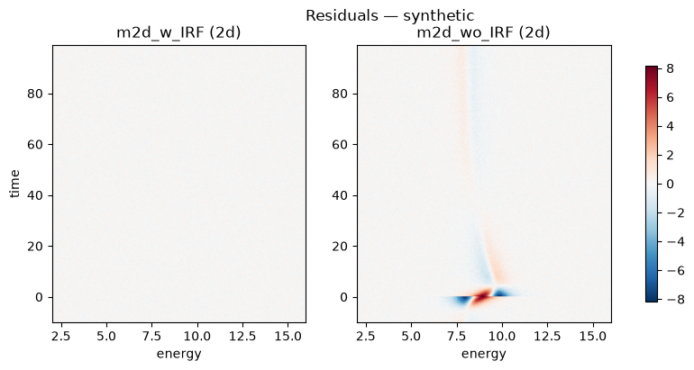
For 2D fits plot_residuals shows the residual maps side by side on a shared diverging scale — it skips the data/fit panels (they look near-identical here). This is the picture behind the AIC/BIC verdict above: m2d_wo_IRF leaves a structured residual band around the t ≈ 0 onset it can’t reproduce, while m2d_w_IRF looks noise-like.
# residual maps of the two 2D fits on one shared color scale
project.results.plot_residuals(
    file=file,
    models=["m2d_w_IRF", "m2d_wo_IRF"],
    fit_type="2d",
);
4. Same Model, Different Settings — variants() and diff()#
compare_models answers which model. The next question that comes up is which configuration of this model — m pinned or free, a tighter bound, another seed. Any change to the inputs produces a new entry in the fit history with its own handle (the short id column in compare_models), side by side with the original. An exact re-run (identical inputs) maps back onto the existing entry. Principle 3 of the fit-archive design spells out exactly which inputs distinguish an exact re-run from a new, unique fit.
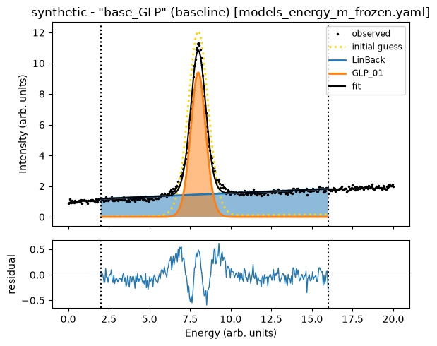
The what-if here: refit base_GLP with the GLP mixing ratio frozen at its YAML seed (m = 0.3; the truth is M_TRUE = 0.85, so the pin is wrong on purpose). A model changes by editing its YAML, so the pinned version lives in a second file, models_energy_m_frozen.yaml, that defines the same base_GLP with m fixed. Loading it under the same model name replaces the live model object — the Model “base_GLP” already exists … overwriting the live model object warning it prints says exactly that; the fits already recorded stay untouched in the history.
# The same base_GLP from a second YAML file, mixing ratio frozen at its 0.3
# seed (reload warning expected): a distinct configuration, not a re-run.
file.load_model(model_yaml="models_energy_m_frozen.yaml", model_info="base_GLP")
file.fit_baseline(model_name="base_GLP", stages=2, try_ci=0)

# Three baseline rows: base_Gauss plus two base_GLP variants — same model
# column, told apart by the handle column.
file.compare_models(fit_type="baseline")
Loading model to describe energy- (and time-)dependent data: base_GLP

Time initialize: 1.1920928955078125e-05 s

Results global minumum fit (method=Nelder):
[[Variables]]
    LinBack_m:       0.04646707 +/- 0.00139528 (3.00%) (init = 0.01)
    LinBack_b:       1.08422737 +/- 0.01433906 (1.32%) (init = 0)
    LinBack_xStart:  0 (fixed)
    LinBack_xStop:   20 (fixed)
    GLP_01_A:        9.39904221 +/- 0.02987925 (0.32%) (init = 12)
    GLP_01_x0:       8.00183927 +/- 0.00164018 (0.02%) (init = 8)
    GLP_01_F:        1.13483833 +/- 0.00472101 (0.42%) (init = 1.5)
    GLP_01_m:        0.3 (fixed)
[[Correlations]] (unreported correlations are < 0.100)
    C(LinBack_m, LinBack_b) = -0.8997
    C(GLP_01_A, GLP_01_F)   = -0.5577
    C(LinBack_b, GLP_01_F)  = -0.2040
Time fit (global minimum): 0.08604264259338379 s

Results local optimization fit (method=leastsq):
[[Variables]]
    LinBack_m:       0.04647226 +/- 0.00139441 (3.00%) (init = 0.01)
    LinBack_b:       1.08420590 +/- 0.01428332 (1.32%) (init = 0)
    LinBack_xStart:  0 (fixed)
    LinBack_xStop:   20 (fixed)
    GLP_01_A:        9.39901560 +/- 0.02899788 (0.31%) (init = 12)
    GLP_01_x0:       8.00183366 +/- 0.00164805 (0.02%) (init = 8)
    GLP_01_F:        1.13482818 +/- 0.00425711 (0.38%) (init = 1.5)
    GLP_01_m:        0.3 (fixed)
[[Correlations]] (unreported correlations are < 0.100)
    C(LinBack_m, LinBack_b) = -0.9006
    C(GLP_01_A, GLP_01_F)   = -0.5182
    C(LinBack_b, GLP_01_F)  = -0.1847
Time fit (local optimization): 0.0029783248901367188 s
Time elapsed for baseline fit: 00.355(ss.ms)
<cell>:3: UserWarning: Model "base_GLP" already exists on file 'synthetic' — replacing the live model object. Completed fits are unaffected (they are kept in the fit history).
  file.load_model(model_yaml="models_energy_m_frozen.yaml", model_info="base_GLP")
| name | value | standard error | relative error | initial value | min | max | vary |
|---|---|---|---|---|---|---|---|
| LinBack_m | 0.04647226 | 0.00139441 | (3.00%) | 0.01 | -1.00000000 | 1.00000000 | True |
| LinBack_b | 1.08420590 | 0.01428332 | (1.32%) | 0.0 | -5.00000000 | 5.00000000 | True |
| LinBack_xStart | 0.00000000 | 0.00000000 | 0.0 | -inf | inf | False | |
| LinBack_xStop | 20.0000000 | 0.00000000 | (0.00%) | 20.0 | -inf | inf | False |
| GLP_01_A | 9.39901560 | 0.02899788 | (0.31%) | 12.0 | 5.00000000 | 15.0000000 | True |
| GLP_01_x0 | 8.00183366 | 0.00164805 | (0.02%) | 8.0 | 5.00000000 | 15.0000000 | True |
| GLP_01_F | 1.13482818 | 0.00425711 | (0.38%) | 1.5 | 0.75000000 | 2.50000000 | True |
| GLP_01_m | 0.30000000 | 0.00000000 | (0.00%) | 0.3 | -inf | inf | False |
| file | model | fit_type | handle | selection_json | chi2_red_raw | sigma_eff | chi2_red | r2 | aic | bic | |
|---|---|---|---|---|---|---|---|---|---|---|---|
| 0 | synthetic | base_Gauss | baseline | 66abe7af | {"base_t_ind": [0, 6], "e_lim": [40, 320]} | 0.051192 | 0.093723 | 5.827871 | 0.988938 | 1612.664494 | 1630.838442 |
| 1 | synthetic | base_GLP | baseline | 0e4fa26e | {"base_t_ind": [0, 6], "e_lim": [40, 320]} | 0.008824 | 0.093723 | 1.004512 | 0.998100 | 287.236404 | 309.045141 |
| 2 | synthetic | base_GLP | baseline | 82c32c49 | {"base_t_ind": [0, 6], "e_lim": [40, 320]} | 0.039654 | 0.093723 | 4.514316 | 0.991431 | 1251.436927 | 1269.610875 |
variants() is the input-side counterpart of compare_models: one (file, model, fit_type) group, one row per run, showing only the input columns that differ — bounds, vary flags, seeds, data corrections. Everything the runs share is suppressed, so the table is the answer to “what did I change between these runs?”.
# the two base_GLP baseline runs: only the inputs that differ are shown
v = project.results.variants(file=file.name, model="base_GLP", fit_type="baseline")
v
| handle | timestamp | GLP_01_m.vary | |
|---|---|---|---|
| 0 | 0e4fa26e | 2026-10-04T04:03:42+00:00 | True |
| 1 | 82c32c49 | 2026-10-04T04:04:00+00:00 | False |
diff(a, b) zooms into one pair: the inputs and fitted values that differ, field by field. Rows for file / model / fit_type appear only when those differ — here both runs are base_GLP baselines, so the table goes straight to the changed input (GLP_01_m.vary) and the fitted values it moved. Fit-quality metrics belong to compare_models and stay out of diff. The 8-character ids from variants() / compare_models are the references — as is a label.
h_free = v.iloc[0]["handle"]     # the §1 fit
h_pinned = v.iloc[-1]["handle"]  # the what-if we just ran
project.results.diff(h_free, h_pinned)
| section | field | 0e4fa26e | 82c32c49 | |
|---|---|---|---|---|
| 0 | input | GLP_01_m.vary | True | False |
| 1 | result | LinBack_m | 0.050349 | 0.046472 |
| 2 | result | LinBack_b | 0.985878 | 1.084206 |
| 3 | result | GLP_01_A | 10.012142 | 9.399016 |
| 4 | result | GLP_01_x0 | 8.001277 | 8.001834 |
| 5 | result | GLP_01_F | 0.997143 | 1.134828 |
| 6 | result | GLP_01_m | 0.858619 | 0.3 |
Close the loop: name the run you keep. set_label writes the archive’s one mutable field — a project-wide unique name that persists through save_fits and works anywhere a handle does. That is what makes selective saving practical: project.save_fits(select=...) takes the same references (handles or labels), so the archive you write holds exactly the runs you mean. The pinned variant stays: distinct configurations are the archive’s record, and notebook 11 uses exactly this group, selecting by the "m-free" label, to show select= choosing among variants.
project.results.set_label(h_free, "m-free") # durable, human-readable pointer
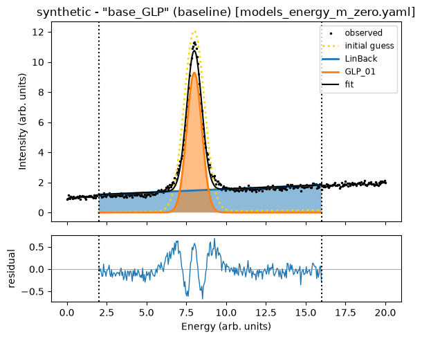
Junk runs are a different matter. Pinning m = 0 looks like a third configuration, but GLP at m = 0 is a pure Gaussian — the same peak base_Gauss already fits, just parametrized by FWHM F instead of SD. The history would hold the same result twice under two model names. Run the mistake anyway, then prune it with drop_fits, which removes the run (and any exact re-runs of it) from the session history.
# The junk what-if: base_GLP with m pinned to 0 (a third YAML file) re-fits
# base_Gauss.
file.load_model(model_yaml="models_energy_m_zero.yaml", model_info="base_GLP")
file.fit_baseline(model_name="base_GLP", stages=2, try_ci=0)

# find() lists a group oldest first, so [-1] is the run just recorded.
junk = project.results.find(
    file=file.name, model="base_GLP", fit_type="baseline"
)[-1]
project.drop_fits(junk.handle)

file.compare_models(fit_type="baseline")  # base_Gauss + the two deliberate variants
Loading model to describe energy- (and time-)dependent data: base_GLP

Time initialize: 1.1444091796875e-05 s

Results global minumum fit (method=Nelder):
[[Variables]]
    LinBack_m:       0.04592078 +/- 0.00139491 (3.04%) (init = 0.01)
    LinBack_b:       1.09821029 +/- 0.01431736 (1.30%) (init = 0)
    LinBack_xStart:  0 (fixed)
    LinBack_xStop:   20 (fixed)
    GLP_01_A:        9.29346134 +/- 0.02950813 (0.32%) (init = 12)
    GLP_01_x0:       8.00191851 +/- 0.00164986 (0.02%) (init = 8)
    GLP_01_F:        1.11065551 +/- 0.00457337 (0.41%) (init = 1.5)
    GLP_01_m:        0 (fixed)
[[Correlations]] (unreported correlations are < 0.100)
    C(LinBack_m, LinBack_b) = -0.9000
    C(GLP_01_A, GLP_01_F)   = -0.5547
    C(LinBack_b, GLP_01_F)  = -0.1994
Time fit (global minimum): 0.07491612434387207 s

Results local optimization fit (method=leastsq):
[[Variables]]
    LinBack_m:       0.04592023 +/- 0.00139389 (3.04%) (init = 0.01)
    LinBack_b:       1.09820452 +/- 0.01425312 (1.30%) (init = 0)
    LinBack_xStart:  0 (fixed)
    LinBack_xStop:   20 (fixed)
    GLP_01_A:        9.29364604 +/- 0.02847041 (0.31%) (init = 12)
    GLP_01_x0:       8.00192215 +/- 0.00164982 (0.02%) (init = 8)
    GLP_01_F:        1.11064333 +/- 0.00402698 (0.36%) (init = 1.5)
    GLP_01_m:        0 (fixed)
[[Correlations]] (unreported correlations are < 0.100)
    C(LinBack_m, LinBack_b) = -0.9011
    C(GLP_01_A, GLP_01_F)   = -0.5062
    C(LinBack_b, GLP_01_F)  = -0.1764
    C(LinBack_b, GLP_01_A)  = -0.1044
Time fit (local optimization): 0.0026693344116210938 s
Time elapsed for baseline fit: 00.347(ss.ms)
Dropped slot 4d68918e (file 'synthetic', model 'base_GLP', baseline): 1 run(s) removed from the in-session history.
<cell>:3: UserWarning: Model "base_GLP" already exists on file 'synthetic' — replacing the live model object. Completed fits are unaffected (they are kept in the fit history).
  file.load_model(model_yaml="models_energy_m_zero.yaml", model_info="base_GLP")
| name | value | standard error | relative error | initial value | min | max | vary |
|---|---|---|---|---|---|---|---|
| LinBack_m | 0.04592023 | 0.00139389 | (3.04%) | 0.01 | -1.00000000 | 1.00000000 | True |
| LinBack_b | 1.09820452 | 0.01425312 | (1.30%) | 0.0 | -5.00000000 | 5.00000000 | True |
| LinBack_xStart | 0.00000000 | 0.00000000 | 0.0 | -inf | inf | False | |
| LinBack_xStop | 20.0000000 | 0.00000000 | (0.00%) | 20.0 | -inf | inf | False |
| GLP_01_A | 9.29364604 | 0.02847041 | (0.31%) | 12.0 | 5.00000000 | 15.0000000 | True |
| GLP_01_x0 | 8.00192215 | 0.00164982 | (0.02%) | 8.0 | 5.00000000 | 15.0000000 | True |
| GLP_01_F | 1.11064333 | 0.00402698 | (0.36%) | 1.5 | 0.75000000 | 2.50000000 | True |
| GLP_01_m | 0.00000000 | 0.00000000 | 0.0 | -inf | inf | False |
| file | model | fit_type | handle | selection_json | chi2_red_raw | sigma_eff | chi2_red | r2 | aic | bic | |
|---|---|---|---|---|---|---|---|---|---|---|---|
| 0 | synthetic | base_Gauss | baseline | 66abe7af | {"base_t_ind": [0, 6], "e_lim": [40, 320]} | 0.051192 | 0.093723 | 5.827871 | 0.988938 | 1612.664494 | 1630.838442 |
| 1 | synthetic | base_GLP | baseline | 0e4fa26e | {"base_t_ind": [0, 6], "e_lim": [40, 320]} | 0.008824 | 0.093723 | 1.004512 | 0.998100 | 287.236404 | 309.045141 |
| 2 | synthetic | base_GLP | baseline | 82c32c49 | {"base_t_ind": [0, 6], "e_lim": [40, 320]} | 0.039654 | 0.093723 | 4.514316 | 0.991431 | 1251.436927 | 1269.610875 |
Tips#
Project.resultsis a property — every access returns a freshFitResultssnapshot. Capture it (r = project.results) to freeze the slot list against subsequent fits, or re-access for the latest view.Handles tie the views together. Every
compare_modelsrow carries a shorthandleid — read them off there or fromvariants(), then feed that 8-character id (or a label) todiff(),set_label(),drop_fits(),select=, and thehandle=kwarg on the single-fit accessors (get_parameters,plot_fit, …).file.compare_models(...)is sugar forproject.results.compare_models(file=file, ...). The implementation lives entirely onFitResults, so loaded archives use the exact same code path.σ is
Filestate, not a per-call argument.compare_models()has nosigma=kwarg by design — column names are stable across calls, sessions, and loaded archives. The σ weights the residual the fit minimizes, so a fit’sstderrfollows from the declared σ.set_sigma()only affects future fits on the file; fits already in the history keep the σ snapshot taken when they completed. For a what-if χ² recalibration of existing results, divide the rawchi2_red_rawcolumn by the alternativesigma_eff**2(for baseline rows that isalt_sigma / √N_avg, squared) — the two-line pandas recipe is in11_save_load_export§1.
Next steps:
See
11_save_load_exportfor the HDF5 round-trip (save_fits/FitResults.load), the matching one-way CSV/PNG export, “ship just the winners” filters, and how to browse a loaded archive.
Model files#
The YAML files next to this notebook, as shipped with the example.
models_energy.yaml#
# Two competing baseline models and two competing SbS models on the same data.
# Each pair deliberately differs in only one structural choice so the
# comparison metrics (chi2_red / r2 / AIC / BIC) have something meaningful
# to say. (available functions: src/trspecfit/functions/energy.py)

# ---- Baseline pair ---------------------------------------------------------
# base_GLP: full GLP profile (Gaussian-Lorentzian product). The simulated data
# was generated with a GLP, so this is the "right" model.
base_GLP:
    LinBack:
      m: [1E-2, True, -1, 1]
      b: [0, True, -5, 5]
      xStart: [0, False]
      xStop: [20, False]
    GLP:
      A: [12, True, 5, 15]
      x0: [8, True, 5, 15]
      F: [1.5, True, 0.75, 2.5]
      m: [0.3, True, 0, 1]

# base_Gauss: pure Gaussian peak (Gauss: A, x0, SD). Same background, one
# structural change: no Lorentzian mixing. One fewer free parameter, but a
# worse fit on data that has Lorentzian tails; AIC/BIC are designed to flag
# exactly this kind of structural underfit.
base_Gauss:
    LinBack:
      m: [1E-2, True, -1, 1]
      b: [0, True, -5, 5]
      xStart: [0, False]
      xStop: [20, False]
    Gauss:
      A: [12, True, 5, 15]
      x0: [8, True, 5, 15]
      SD: [0.6, True, 0.2, 2.5]

# ---- Slice-by-Slice pair ---------------------------------------------------
# sbs_x0_only: only the peak position x0 evolves with time (the truth in the
# simulated data). Background and amplitude pinned from the baseline fit.
sbs_x0_only:
    LinBack:
      m: [1E-2, False]
      b: [0, False]
      xStart: [0, False]
      xStop: [20, False]
    GLP:
      A: [12, False]
      x0: [8, True, 5, 15]
      F: [1.5, False]
      m: [0.3, False]

# sbs_x0_A: x0 AND A both vary per slice. More flexible: the raw chi2 drops on
# nearly every slice, but chi2_red, AIC and BIC charge for the extra free
# parameter and favour it on only a minority of slices.
sbs_x0_A:
    LinBack:
      m: [1E-2, False]
      b: [0, False]
      xStart: [0, False]
      xStop: [20, False]
    GLP:
      A: [12, True, 5, 15]
      x0: [8, True, 5, 15]
      F: [1.5, False]
      m: [0.3, False]

# ---- 2D pair ---------------------------------------------------------------
# m2d_w_IRF / m2d_wo_IRF share an identical energy model (LinBack + GLP, all
# pinned from baseline). They differ only in which dynamics model gets
# attached to x0 via `file.add_time_dependence(...)`:
#   m2d_w_IRF -> MonoExpPosIRF  (shift-and-decay convolved with a Gaussian IRF)
#   m2d_wo_IRF -> MonoExpPos     (sharp shift-and-decay, no IRF)
# The simulated data was generated with an IRF-smeared shift-and-decay, so we
# expect m2d_w_IRF to win even after AIC/BIC penalize its extra free
# parameter (the IRF σ).
m2d_w_IRF:
    LinBack:
      m: [1E-2, False]
      b: [0, False]
      xStart: [0, False]
      xStop: [20, False]
    GLP:
      A: [12, False]
      x0: [8, True, 5, 15]
      F: [1.5, False]
      m: [0.3, False]

m2d_wo_IRF:
    LinBack:
      m: [1E-2, False]
      b: [0, False]
      xStart: [0, False]
      xStop: [20, False]
    GLP:
      A: [12, False]
      x0: [8, True, 5, 15]
      F: [1.5, False]
      m: [0.3, False]
models_energy_m_frozen.yaml#
# Section 4 of the notebook: the same base_GLP as in models_energy.yaml with
# the GLP mixing ratio frozen at its seed. A model changes by editing the
# YAML and reloading, so a pinned variant is a second file that defines the
# same model name; loaded under that name it is a distinct configuration of
# base_GLP, not a new model.
base_GLP:
    LinBack:
      m: [1E-2, True, -1, 1]
      b: [0, True, -5, 5]
      xStart: [0, False]
      xStop: [20, False]
    GLP:
      A: [12, True, 5, 15]
      x0: [8, True, 5, 15]
      F: [1.5, True, 0.75, 2.5]
      m: [0.3, False]
models_energy_m_zero.yaml#
# Section 4 of the notebook, the junk what-if: base_GLP with the mixing ratio
# pinned to 0, which makes the GLP a pure Gaussian and re-fits what base_Gauss
# already fits. Same model name as models_energy.yaml, so it lands as a
# variant of base_GLP and is then dropped.
base_GLP:
    LinBack:
      m: [1E-2, True, -1, 1]
      b: [0, True, -5, 5]
      xStart: [0, False]
      xStop: [20, False]
    GLP:
      A: [12, True, 5, 15]
      x0: [8, True, 5, 15]
      F: [1.5, True, 0.75, 2.5]
      m: [0, False]
models_time.yaml#
# Time-domain dynamics models for `file.add_time_dependence(...)`.
# (available functions: src/trspecfit/functions/time.py)

# MonoExpPosIRF — shift-and-decay smeared by a Gaussian instrument response.
# Matches the simulated ground truth in this notebook (IRF σ ≈ 3, τ ≈ 30).
MonoExpPosIRF:
    gaussCONV:
        SD: [3, True, 1.0E-6, 10]
    expFun:
        A: [2, True, 0, 10]
        tau: [30, True, 1, 100]
        t0: [0, False]

# MonoExpPos — same shift-and-decay, no IRF convolution. Sharp turn-on
# at t = t0; will undershoot the smoothed onset around t = 0.
MonoExpPos:
    expFun:
        A: [2, True, 0, 10]
        tau: [30, True, 1, 100]
        t0: [0, False]
project.yaml#
# Project configuration for the model-comparison example

# Display settings
show_output: 1

# Axis labels
e_label: 'Energy (arb. units)'
t_label: 'Time (arb. units)'
z_label: 'Intensity (arb. units)'

# Plot settings
x_dir: 'def'
x_type: 'lin'
y_dir: 'def'
y_type: 'lin'
z_colormap: 'viridis'
z_type: 'lin'
dpi_plt: 100
dpi_save: 300
res_mult: 5