Uncertainty Estimation Overview#
Error bars are estimates made under a model — and they depend on the noise model as much as on the fit model. Declare the noise once and every later fit on that file minimizes the matching likelihood, so stderr, confidence intervals and MCMC widths all mean the same ±1σ. This notebook re-runs 01_basic_fitting, declares the photon-counting noise its data carry, and works through the three tiers of uncertainty estimation trspecfit exposes. The tiers are ordered by computational cost: each one assumes less than the last, but takes longer to run. Usually you want the cheapest tier that is still valid for your case.
Tier |
Access via |
Comes from |
Extra cost |
Characteristic failure |
|---|---|---|---|---|
#1 |
|
covariance matrix at the fit minimum |
none, a byproduct of the fit |
non-quadratic χ² surface: a bound within a few σ, a curved valley, a near-degeneracy |
#2 |
|
χ² profiling ( |
dozens of re-fits per free parameter |
parameters at/near bounds |
#3 |
|
MCMC posterior sampling ( |
|
unconverged chains |
Notebook 01’s data is synthetic and ships with truth YAMLs, so the error bars can be checked against the known answer — and against the Cramér-Rao bound, the smallest uncertainty the photon budget allows.
Workflow:
Re-run example 01: its fits and synthetic data are what this notebook builds on.
Declare the noise model: one
set_noiseline for counting data, and the χ²_red ≈ 1 gate that checks it.Create and review all three uncertainty estimates: Run a baseline fit with
stderr(free),try_ci=1(profiled CIs), and MCMC (mc_settings). Read fit results back with theget_*accessors —get_parameters/get_correlations(tier 1),get_confidence_intervals(tier 2),get_mcmc(tier 3), withplot_mcmcfor the chain diagnostics — and walk through the assumptions behind each tier.Compare each result against the truth and the bound: the three tiers side by side with the known answer and with
sensitivity.crb, the Cramér-Rao bound at this photon budget.Scale up to the 2D fit: the same deliberately short chain on the global fit, and how to read its convergence diagnostics.
0. Re-run Example Notebook 01#
%%capture
# %%capture swallows notebook 01's plots/output

# %cd into notebook 01's dir so its project.yaml + data/models resolve
%cd -q "../01_basic_fitting"
# %run executes that notebook in the current kernel (variables stay live)
%run example.ipynb
# %cd - returns here
%cd -q -
# Sanity check: notebook 01 should have left one File with a fitted baseline
# model (6 free parameters) and a fitted 2D model (4 free parameters) in scope.
n_free_base = sum(level != "static" for level in file.model_base.get_vary_levels().values())
n_free_2d = sum(level != "static" for level in file.model_2d.get_vary_levels().values())
assert (n_free_base, n_free_2d) == (6, 4), "notebook 01 did not run to completion"
print(f"OK: file {file.name!r} carries {file.model_base.name!r} ({n_free_base} free) "
      f"and {file.model_2d.name!r} ({n_free_2d} free)")
OK: file 'data' carries 'base' (6 free) and '2D' (4 free)
import numpy as np
import pandas as pd
import trspecfit
from ruamel.yaml import YAML

from trspecfit import sensitivity
from trspecfit.utils.lmfit import MC
# helper: 1-sigma half-width per parameter from a CI / quantile table
def one_sigma_halfwidth(ci_df):
    half = (ci_df["+1.0"] - ci_df["-1.0"]) / 2
    return dict(zip(ci_df["par[v]/sigma[>]"], half))
1. Declare the Noise Model#
An error bar answers “how far can this parameter move before the data stop supporting it”, and that question has no answer until the noise is named. Notebook 01’s data come from a photon-counting simulation: data/generate_data.ipynb runs Simulator(detection='photon_counting', counts_per_delay=5000). Every pixel is therefore a Poisson draw whose variance is its own count, and file.set_noise("poisson", scale=...) says exactly that.
scale is counts per data unit. The generator scaled the clean signal so that the mean time slice carries its 5000-count budget, drew the counts, and divided them back by that factor, so the stored data are in model units and the scale has to be handed back. Data that already are counts need nothing — scale=1 is the default.
The declaration is file state: every fit from here on minimizes the Poisson deviance, and stderr, the profiled intervals and the posterior all come out in units of that noise. It is also checkable. A fit whose residuals are the size the declared noise predicts has chi2_red ≈ 1, and §2 reads that gate straight after the fit. The metric is proportional to the declared scale, so a mis-stated photon budget lands somewhere other than 1.
What the default — no declaration, noise_type='unknown' — does to the same fit is 13_missing_noise_model.
# counts per data unit: the generator spent 5000 counts on the mean time slice,
# so dividing by the mean slice total of the stored data recovers its factor
scale = 5000 / file.data.sum(axis=1).mean()
file.set_noise("poisson", scale=scale)  # weights every later fit on this file
print(f"scale = {scale:.2f} counts per data unit")
scale = 3.65 counts per data unit
2. One Fit, All Tiers#
In practice you would start with the cheapest estimate and move to a more expensive tier only if you need to. Here a single baseline fit turns on all three at once, and the declared noise changes what each of them means:
stderr— the curvature of the weighted χ² at the minimum (Nonewhen lmfit cannot invert that curvature matrix). lmfit no longer rescales the covariance to force χ²_red = 1, so the error bar follows the declared noise instead of the residual scatter.try_ci=1— profiled confidence intervals fromlmfit.conf_interval, thresholded on χ². Its default F-test profiles out a noise scale the declaration already fixes, so the two thresholds agree only where χ²_red is 1 anyway.mc_settings— posterior sampling withlmfit.emcee. The residual is already in units of σ, so emcee samples the posterior itself: there is no__lnsigmanuisance parameter riding along with the model parameters, and no starting noise scale to get wrong.nwalkersdefaults to 2 × free parameters with a floor of 20, and the floor is what governs here.
Two settings carry the chain. steps should reach 50 × the chain’s autocorrelation time τ — below that emcee warns it cannot estimate τ reliably (§4 runs into it on purpose) — and burn discards the burn-in. seed makes the chain reproducible; the fit itself does not depend on it.
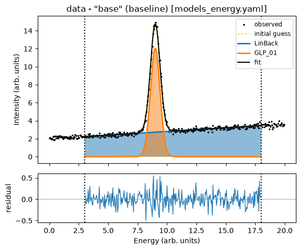
Everything below reads off this single fit through the get_* accessors; nothing is re-fit. The fit prints a lot at once (the Bound reached warning, the emcee progress bar, the corner and acceptance plots), and the next sections take it one tier at a time.
mc = MC(
    use_mc=1,  # 1: always sample (2 would sample only if conf_interval fails)
    steps=6000,  # >= 50x the autocorrelation time (emcee warns below if not)
    burn=600,  # discard the burn-in
    seed=1,  # reproducible chain; nwalkers is derived
)
# one fit, all three methods: leastsq stderr + profiled CIs + MCMC posterior
file.fit_baseline(model_name="base", stages=2, try_ci=1, mc_settings=mc)
Time initialize: 1.3113021850585938e-05 s

Results global minumum fit (method=Nelder):
[[Variables]]
    LinBack_m:       0.08169647 +/- 0.00182975 (2.24%) (init = 0.08178437)
    LinBack_b:       1.98921975 +/- 0.02059116 (1.04%) (init = 1.987888)
    LinBack_xStart:  0 (fixed)
    LinBack_xStop:   20 (fixed)
    GLP_01_A:        12.0505830 +/- 0.11154573 (0.93%) (init = 12.05968)
    GLP_01_x0:       9.00081020 +/- 0.00299882 (0.03%) (init = 9.001392)
    GLP_01_F:        0.99404444 +/- 0.00702310 (0.71%) (init = 0.9939177)
    GLP_01_m:        0.21907778 +/- 0.07142858 (32.60%) (init = 0.2329643)
[[Correlations]] (unreported correlations are < 0.100)
    C(LinBack_m, LinBack_b) = -0.9048
    C(GLP_01_A, GLP_01_F)   = -0.6386
    C(GLP_01_A, GLP_01_m)   = +0.5494
    C(GLP_01_F, GLP_01_m)   = -0.3099
    C(LinBack_b, GLP_01_m)  = -0.1204
Time fit (global minimum): 0.12998032569885254 s

Results local optimization fit (method=leastsq):
[[Variables]]
    LinBack_m:       0.08169650 +/- 0.00183037 (2.24%) (init = 0.08178437)
    LinBack_b:       1.98921915 +/- 0.02059166 (1.04%) (init = 1.987888)
    LinBack_xStart:  0 (fixed)
    LinBack_xStop:   20 (fixed)
    GLP_01_A:        12.0505909 +/- 0.11130011 (0.92%) (init = 12.05968)
    GLP_01_x0:       9.00080949 +/- 0.00299910 (0.03%) (init = 9.001392)
    GLP_01_F:        0.99404492 +/- 0.00702388 (0.71%) (init = 0.9939177)
    GLP_01_m:        0.21907572 +/- 0.07061732 (32.23%) (init = 0.2329643)
[[Correlations]] (unreported correlations are < 0.100)
    C(LinBack_m, LinBack_b) = -0.9049
    C(GLP_01_A, GLP_01_F)   = -0.6391
    C(GLP_01_A, GLP_01_m)   = +0.5468
    C(GLP_01_F, GLP_01_m)   = -0.3111
    C(LinBack_b, GLP_01_m)  = -0.1178
Time fit (local optimization): 0.0030002593994140625 s

              99.73%    95.45%    68.27%    _BEST_    68.27%    95.45%    99.73%
 LinBack_m:  -0.00549  -0.00366  -0.00183   0.08170  +0.00183  +0.00366  +0.00549
 LinBack_b:  -0.06152  -0.04107  -0.02056   1.98922  +0.02062  +0.04129  +0.06203
 GLP_01_A :  -0.32693  -0.21979  -0.11074  12.05059  +0.11232  +0.22613  +0.34141
 GLP_01_x0:  -0.00900  -0.00601  -0.00300   9.00081  +0.00300  +0.00600  +0.00900
 GLP_01_F :  -0.02444  -0.01536  -0.00727   0.99404  +0.00692  +0.01376  +0.02061
 GLP_01_m :      -inf      -inf  -0.07952   0.21908  +0.06635  +0.12503  +0.17810

Progress of lmfit.emcee confidence interval determination
(based on Markov chain Monte Carlo parameter space sampling):

Results lmfit.emcee() confidence interval determination:
[[Variables]]
    LinBack_m:       0.08176014 +/- 0.00184839 (2.26%) (init = 0.0816965)
    LinBack_b:       1.98926005 +/- 0.02047750 (1.03%) (init = 1.989219)
    LinBack_xStart:  0 (fixed)
    LinBack_xStop:   20 (fixed)
    GLP_01_A:        12.0413428 +/- 0.11149336 (0.93%) (init = 12.05059)
    GLP_01_x0:       9.00072061 +/- 0.00300754 (0.03%) (init = 9.000809)
    GLP_01_F:        0.99218187 +/- 0.00733065 (0.74%) (init = 0.9940449)
    GLP_01_m:        0.20493091 +/- 0.07942475 (38.76%) (init = 0.2190757)
[[Correlations]] (unreported correlations are < 0.100)
    C(LinBack_m, LinBack_b) = -0.9024
    C(GLP_01_A, GLP_01_m)   = +0.5521
    C(GLP_01_A, GLP_01_F)   = -0.4542
    C(LinBack_b, GLP_01_F)  = -0.1116
Time lmfit.emcee: 20.028480291366577 s
None
Time elapsed for baseline fit: 24.686(ss.ms)
<site-packages>/lmfit/confidence.py:356: UserWarning: Bound reached with prob(GLP_01_m=0) = 0.9466414609858015 < max(sigmas)
  warn(errmsg)
100%|██████████| 6000/6000 [00:19<00:00, 301.51it/s]
| par[v]/sigma[>] | -3.0 | -2.0 | -1.0 | best fit | +1.0 | +2.0 | +3.0 | |
|---|---|---|---|---|---|---|---|---|
| 0 | LinBack_m | 0.076251 | 0.078060 | 0.079845 | 0.081760 | 0.083543 | 0.085397 | 0.087086 |
| 1 | LinBack_b | 1.927268 | 1.948449 | 1.968873 | 1.989260 | 2.009843 | 2.030332 | 2.049449 |
| 2 | GLP_01_A | 11.712097 | 11.822218 | 11.931227 | 12.041343 | 12.154220 | 12.263147 | 12.376956 |
| 3 | GLP_01_x0 | 8.991958 | 8.994735 | 8.997773 | 9.000721 | 9.003789 | 9.006756 | 9.009788 |
| 4 | GLP_01_F | 0.967575 | 0.976482 | 0.984662 | 0.992182 | 0.999326 | 1.006530 | 1.013579 |
| 5 | GLP_01_m | 0.001201 | 0.025062 | 0.116224 | 0.204931 | 0.275100 | 0.335030 | 0.386166 |
| name | value | standard error | relative error | initial value | min | max | vary |
|---|---|---|---|---|---|---|---|
| LinBack_m | 0.08169650 | 0.00183037 | (2.24%) | 0.0817843707272019 | -1.00000000 | 1.00000000 | True |
| LinBack_b | 1.98921915 | 0.02059166 | (1.04%) | 1.987888192824693 | -5.00000000 | 5.00000000 | True |
| LinBack_xStart | 0.00000000 | 0.00000000 | 0.0 | -inf | inf | False | |
| LinBack_xStop | 20.0000000 | 0.00000000 | (0.00%) | 20.0 | -inf | inf | False |
| GLP_01_A | 12.0505909 | 0.11130011 | (0.92%) | 12.059676813726696 | 5.00000000 | 15.0000000 | True |
| GLP_01_x0 | 9.00080949 | 0.00299910 | (0.03%) | 9.001392138494767 | 5.00000000 | 15.0000000 | True |
| GLP_01_F | 0.99404492 | 0.00702388 | (0.71%) | 0.9939177030931372 | 0.75000000 | 2.50000000 | True |
| GLP_01_m | 0.21907572 | 0.07061732 | (32.23%) | 0.23296426434035067 | 0.00000000 | 1.00000000 | True |
# the gate for this fit: chi2_red against the declared noise. The file carries
# notebook 01's baseline fit too, made before the declaration, so read the slot
# this fit just wrote rather than a table spanning two noise models.
slot_base = project.results.find(file=file.name, fit_type="baseline")[-1]
chi2_red = slot_base.metrics["chi2_red"]
print(f"chi2_red = {chi2_red:.2f}  (1 = residuals the size the noise predicts)")
chi2_red = 1.06 (1 = residuals the size the noise predicts)
2.1 Tier 1 — stderr: the Free Error Bar#
A leastsq fit reports a stderr per parameter from the covariance matrix (inverse Hessian) at the minimum, or None when that matrix cannot be inverted. One assumption is left in it: the χ² surface is quadratic near the minimum. That is always true close enough to the minimum; the question is whether ±1σ is still close. The other assumption an unweighted fit has to make — that the residual scatter is the noise — is the one §1 removed.
stderr is a marginal width: the covariance already accounts for the other parameters moving, so a strong correlation by itself does not make it wrong. The most strongly correlated pair in the matrix below, LinBack_m and LinBack_b, get matching stderr, profiled and MCMC widths in §3. What the correlation matrix from get_correlations tells you is which parameters trade off: their joint confidence region is a tilted ellipse, not the box the two stderr values suggest, and fixing one would shrink the other’s error bar.
Where the surface stops being quadratic, the covariance no longer describes it and stderr stops meaning ±1σ. The tier table in the opening lists the three ways that happens. Notebook 04_parameter_profiles meets an exact degeneracy and fixes the IMFP from tables rather than fitting it.
# stderr is the free byproduct of the leastsq covariance (one row per par)
file.get_parameters(fit_type="baseline")[["name", "value", "stderr", "vary"]]
| name | value | stderr | vary | |
|---|---|---|---|---|
| 0 | LinBack_m | 0.081697 | 0.001830 | True |
| 1 | LinBack_b | 1.989219 | 0.020592 | True |
| 2 | LinBack_xStart | 0.000000 | 0.000000 | False |
| 3 | LinBack_xStop | 20.000000 | 0.000000 | False |
| 4 | GLP_01_A | 12.050591 | 0.111300 | True |
| 5 | GLP_01_x0 | 9.000809 | 0.002999 | True |
| 6 | GLP_01_F | 0.994045 | 0.007024 | True |
| 7 | GLP_01_m | 0.219076 | 0.070617 | True |
# who trades off against whom: the correlation matrix
file.get_correlations(fit_type="baseline").round(2)
| LinBack_m | LinBack_b | GLP_01_A | GLP_01_x0 | GLP_01_F | GLP_01_m | |
|---|---|---|---|---|---|---|
| LinBack_m | 1.00 | -0.90 | 0.03 | -0.04 | 0.04 | 0.05 |
| LinBack_b | -0.90 | 1.00 | -0.08 | 0.03 | -0.09 | -0.12 |
| GLP_01_A | 0.03 | -0.08 | 1.00 | -0.00 | -0.64 | 0.55 |
| GLP_01_x0 | -0.04 | 0.03 | -0.00 | 1.00 | 0.01 | 0.00 |
| GLP_01_F | 0.04 | -0.09 | -0.64 | 0.01 | 1.00 | -0.31 |
| GLP_01_m | 0.05 | -0.12 | 0.55 | 0.00 | -0.31 | 1.00 |
2.2 Tier 2 — try_ci=1: Profiled Confidence Intervals#
try_ci=1 runs lmfit.conf_interval: it walks each parameter away from the optimum, re-optimizing all the others, until the weighted χ² has risen past the threshold for the requested confidence level. No quadratic assumption, and the intervals come out asymmetric, reported at the levels in ci_sigmas (default [1, 2, 3]).
The fit above printed a Bound reached warning, and that is tier 2’s failure mode. The Lorentzian fraction GLP_01_m has a hard lower bound at 0, and its −2σ and −3σ profile excursions run into it: lmfit warns Bound reached with prob(GLP_01_m=0) ... < max(sigmas) and reports -inf for those entries. A profiled CI isn’t defined past a parameter bound. The other notebooks pass try_ci=0 and point here; this is the failure mode they left for this one. The MCMC posterior in the next section handles the same bound without breaking.
# tier 2: the profiled CI table (note the -inf where the GLP_01_m profile hit 0)
ci_table = file.get_confidence_intervals(fit_type="baseline")
ci_table
| par[v]/sigma[>] | -3.0 | -2.0 | -1.0 | best fit | +1.0 | +2.0 | +3.0 | |
|---|---|---|---|---|---|---|---|---|
| 0 | LinBack_m | 0.076204 | 0.078035 | 0.079866 | 0.081697 | 0.083526 | 0.085354 | 0.087182 |
| 1 | LinBack_b | 1.927698 | 1.948149 | 1.968656 | 1.989219 | 2.009839 | 2.030514 | 2.051245 |
| 2 | GLP_01_A | 11.723657 | 11.830798 | 11.939848 | 12.050591 | 12.162909 | 12.276723 | 12.392002 |
| 3 | GLP_01_x0 | 8.991811 | 8.994803 | 8.997811 | 9.000809 | 9.003809 | 9.006808 | 9.009807 |
| 4 | GLP_01_F | 0.969603 | 0.978687 | 0.986776 | 0.994045 | 1.000965 | 1.007806 | 1.014650 |
| 5 | GLP_01_m | -inf | -inf | 0.139559 | 0.219076 | 0.285424 | 0.344107 | 0.397176 |
2.3 Tier 3 — MCMC: Reading the Posterior#
MCMC isn’t a fit; it samples the posterior around the converged solution, so correlations, asymmetries, and tails clipped at bounds all show up directly. get_mcmc returns the sampled chain, the per-walker acceptance fractions and the posterior quantile table — one row per varying model parameter and nothing else, because the declared noise leaves no nuisance parameter to sample.
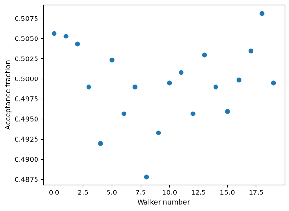
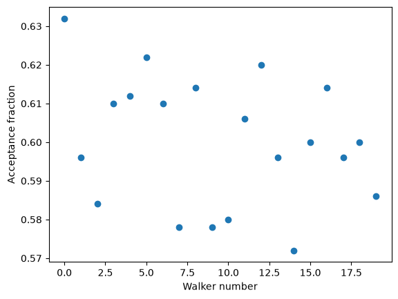
Acceptance fraction — the share of proposals the walkers took. Near 0 they are stuck and nothing is being sampled; emcee’s rule of thumb is 0.2–0.5, and its stretch move sits at the top of that range or above it in few dimensions. It checks mixing, not convergence (§4).
The resolved settings the fit recorded say what actually ran: the derived
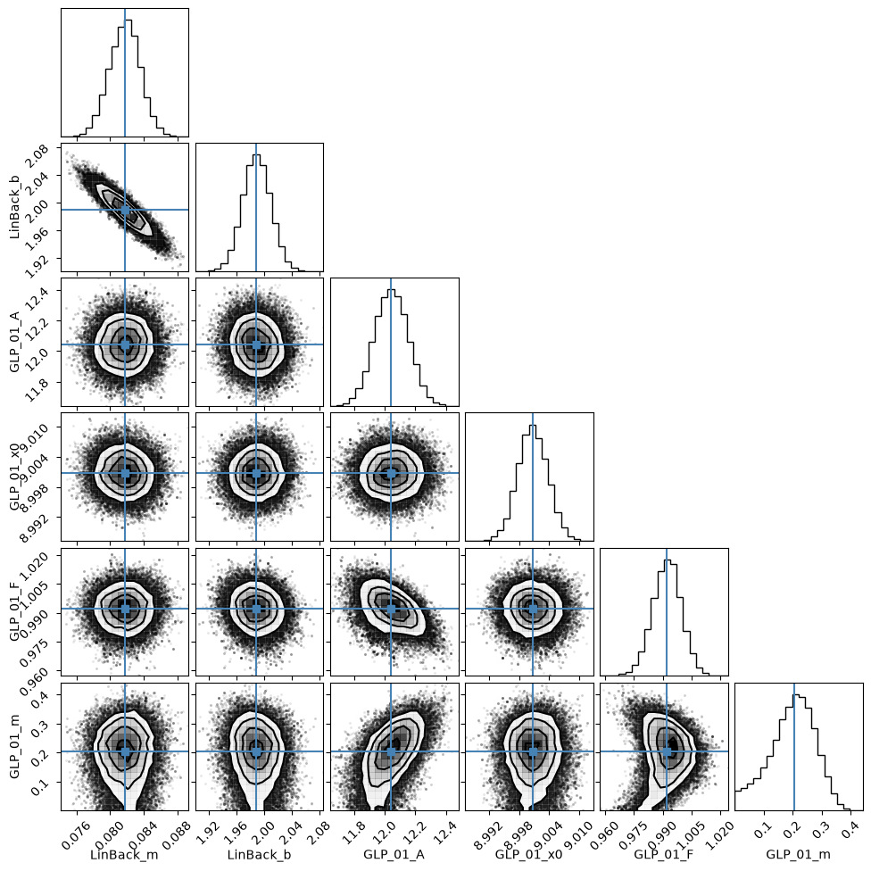
nwalkers,is_weightedtrue, and no σ knobs at all — there is no noise scale to start, bound or sample.The corner plot (re-rendered below from the saved chain) shows the pairwise marginals. The tilted ellipse of
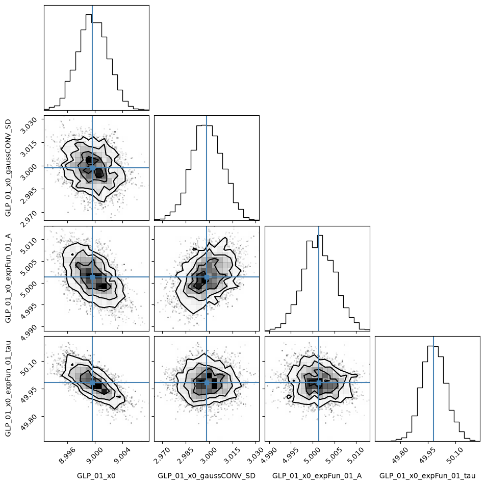
LinBack_magainstLinBack_bis their strong correlation. The bentGLP_01_F/GLP_01_mpanel is a non-quadratic surface, tier 1’s real failure mode. The lower tail ofGLP_01_mis clipped at its 0 bound, so tier 3 reports a finite −3σ quantile where tier 2 returned-inf.
mcmc = file.get_mcmc(fit_type="baseline")

print(f"acceptance fraction: {mcmc.acceptance_fraction.mean():.2f}")
# what ran: knobs left at None appear in the slot's provenance with the values
# the fit derived for them
print(f"resolved MC settings: {slot_base.fit_settings['mc']}")
acceptance fraction: 0.50
resolved MC settings: {'use_mc': 1, 'steps': 6000, 'nwalkers': 20, 'burn': 600, 'thin': 1, 'ntemps': 1, 'is_weighted': True, 'seed': 1}
# tier 3: the posterior quantile table
mcmc.table
| par[v]/sigma[>] | -3.0 | -2.0 | -1.0 | best fit | +1.0 | +2.0 | +3.0 | |
|---|---|---|---|---|---|---|---|---|
| 0 | LinBack_m | 0.076251 | 0.078060 | 0.079845 | 0.081760 | 0.083543 | 0.085397 | 0.087086 |
| 1 | LinBack_b | 1.927268 | 1.948449 | 1.968873 | 1.989260 | 2.009843 | 2.030332 | 2.049449 |
| 2 | GLP_01_A | 11.712097 | 11.822218 | 11.931227 | 12.041343 | 12.154220 | 12.263147 | 12.376956 |
| 3 | GLP_01_x0 | 8.991958 | 8.994735 | 8.997773 | 9.000721 | 9.003789 | 9.006756 | 9.009788 |
| 4 | GLP_01_F | 0.967575 | 0.976482 | 0.984662 | 0.992182 | 0.999326 | 1.006530 | 1.013579 |
| 5 | GLP_01_m | 0.001201 | 0.025062 | 0.116224 | 0.204931 | 0.275100 | 0.335030 | 0.386166 |
# MCMC diagnostics re-rendered from the saved fit slot: walker acceptance + corner
file.plot_mcmc(fit_type="baseline")
3. The Three Tiers Side by Side — Truth and the Bound#
One row per free parameter: the ±1σ half-widths from all three tiers, the truth value from notebook 01’s data/models_energy_truth.yaml, the pull (fit − truth)/stderr, and the Cramér-Rao bound. That bound is the smallest standard deviation any unbiased estimator can reach on this model shape with this many photons. sensitivity.crb computes it from the model alone, so it is an outside yardstick: no fit, no data.
The bound needs the photon budget of the fitted view. The baseline fit is the mean of the pre-t0 slices over the energy window, and a sum of Poisson draws is Poisson, so that mean carries n_avg times the per-slice counts. Evaluating the truth model on the same energy window and multiplying its total by scale × n_avg gives the counts the fit had to work with.
Three things to check:
The tiers agree.
LinBack_mandLinBack_bare strongly correlated and still get the same ±1σ fromstderr, the profiled CI and the MCMC quantiles: correlation alone costs tier 1 nothing. The widest spread is onGLP_01_m, whose posterior is clipped at its 0 bound. When the tiers agree, the cheapest one is all you need.stderrsits on the bound. With the noise declared, the fit minimizes the exact counting likelihood, and its error bars land on the smallest ones the photon budget allows.GLP_01_FandGLP_01_mare the two that differ: the bound is evaluated at the truth and the covariance at the fitted values, and the peak’s information about its width and its mixing fraction both depend on the mixing fraction, which the fit places below the truth.The pulls are O(1). All six sit within one σ of the truth, so the error bars are calibrated: they cover the true values at the rate they claim, not merely self-consistently. (One six-parameter draw is a spot check, not a proof, but a pull of 5 would tell you something is off.)
# truth values, read via ruamel (the project's YAML stack, same as load_model)
# so scientific-notation scalars like 8E-2 parse as floats.
truth_yaml_name = "data/models_energy_truth.yaml"  # resolved against project.path
truth_yaml = YAML(typ="safe").load(project.path / truth_yaml_name)["base"]
truth = {f"LinBack_{k}": v[0] for k, v in truth_yaml["LinBack"].items()}
truth |= {f"GLP_01_{k}": v[0] for k, v in truth_yaml["GLP"].items()}
# the bound wants a model on the axis that was fitted, so put the truth model on
# the energy window: a File is how an axis and a model come together.
e0, e1 = file.e_lim
n_avg = file.base_t_ind[1] - file.base_t_ind[0]  # slices the baseline averaged
truth_file = trspecfit.File(
    parent_project=project,
    name="truth",  # a second file in the project needs its own name
    energy=file.energy[e0:e1],
)
truth_file.load_model(model_yaml=truth_yaml_name, model_info="base")
truth_model = truth_file.model_active

truth_curve = truth_model.create_value_1d(return_1d=1)  # 1: hand the array back
counts = scale * n_avg * truth_curve.sum()
# the fit holds the background clamp fixed, so the bound spans the same free
# parameters: fixed= treats them as known without touching the truth model
bound = sensitivity.crb(
    truth_model, counts=counts, fixed=("LinBack_xStart", "LinBack_xStop")
)
print(f"photon budget of the baseline fit: {counts:,.0f} counts")
Loading model to describe energy- (and time-)dependent data: base
photon budget of the baseline fit: 165,532 counts
# one row per free model parameter: each tier's 1-sigma half-width, the bound,
# the truth and the pull. All three tiers come from the one baseline fit.
fit_df = file.get_parameters(fit_type="baseline").set_index("name")
ci_1s = one_sigma_halfwidth(ci_table)
mcmc_1s = one_sigma_halfwidth(mcmc.table)
rows = [
    {
        "parameter": name,
        "truth": truth[name],
        "fit": row["value"],
        "stderr": row["stderr"],
        "ci_1sigma": ci_1s[name],
        "mcmc_1sigma": mcmc_1s[name],
        "crb": bound[name],
        "pull": (row["value"] - truth[name]) / row["stderr"],
    }
    for name, row in fit_df.iterrows()
    if row["vary"] and name in truth
]
pd.DataFrame(rows).round(4)
| parameter | truth | fit | stderr | ci_1sigma | mcmc_1sigma | crb | pull | |
|---|---|---|---|---|---|---|---|---|
| 0 | LinBack_m | 0.08 | 0.0817 | 0.0018 | 0.0018 | 0.0018 | 0.0018 | 0.9269 |
| 1 | LinBack_b | 2.00 | 1.9892 | 0.0206 | 0.0206 | 0.0205 | 0.0206 | -0.5236 |
| 2 | GLP_01_A | 12.00 | 12.0506 | 0.1113 | 0.1115 | 0.1115 | 0.1114 | 0.4545 |
| 3 | GLP_01_x0 | 9.00 | 9.0008 | 0.0030 | 0.0030 | 0.0030 | 0.0030 | 0.2699 |
| 4 | GLP_01_F | 1.00 | 0.9940 | 0.0070 | 0.0071 | 0.0073 | 0.0077 | -0.8478 |
| 5 | GLP_01_m | 0.25 | 0.2191 | 0.0706 | 0.0729 | 0.0794 | 0.0660 | -0.4379 |
4. Scaling Up: MCMC on the 2D Fit#
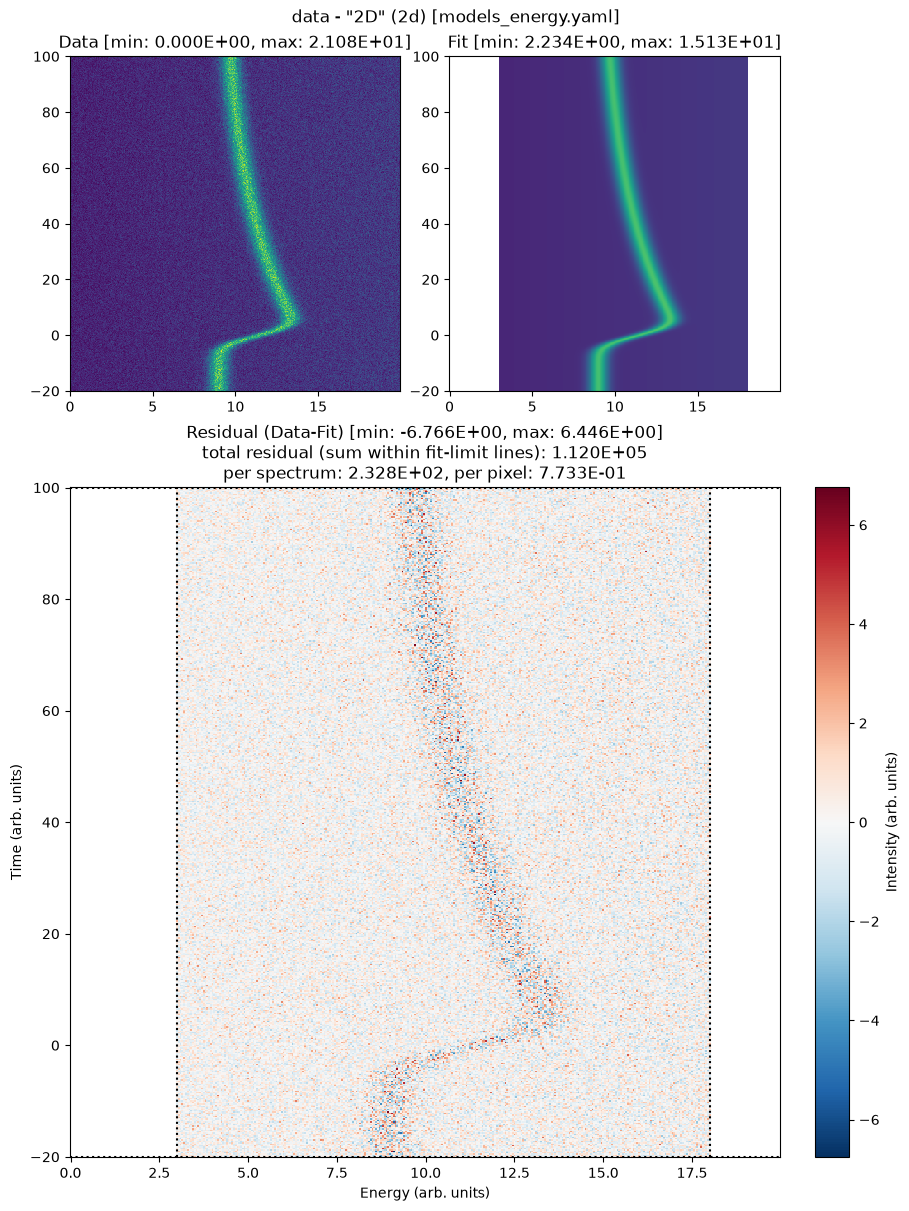
The same call works on the global 2D fit; only the cost changes, since every posterior sample now evaluates the full 2D model. To keep the notebook fast we run a deliberately short chain of 500 steps. The autocorrelation time τ here is tens of steps (the printout lists them), so emcee prints “The chain is shorter than 50 times the integrated autocorrelation time”. That warning says emcee cannot vouch for its own τ estimate. It does not say whether the walkers reached the posterior, and neither does the acceptance fraction.
What settles it is tier 1. Away from bounds the posterior width and stderr measure the same curvature, so a short chain that has arrived reproduces them parameter by parameter; the table below checks that. A chain that has not arrived returns confidently wrong widths while its own diagnostics look unchanged — 13_missing_noise_model runs that control.
mc_2d = MC(
    use_mc=1,  # as in §2: always sample
    steps=500,  # deliberately short: well under 50x tau, so emcee warns
    burn=100,  # discard the burn-in
    seed=1,  # reproducible chain
)
# same call on the global 2D model: every posterior sample evaluates the full 2D
# fit. stages=2 ends in leastsq, so the stderr the chain is compared with below
# is tier 1 as §2 defined it; try_ci=0 because the chain covers tier 2.
file.fit_2d(model_name="2D", stages=2, try_ci=0, mc_settings=mc_2d)
Time initialize: 1.2159347534179688e-05 s

Results global minumum fit (method=Nelder):
[[Variables]]
    LinBack_m:                0.0816965 (fixed)
    LinBack_b:                1.989219 (fixed)
    LinBack_xStart:           0 (fixed)
    LinBack_xStop:            20 (fixed)
    GLP_01_A:                 12.05059 (fixed)
    GLP_01_x0:                8.99966079 +/- 0.00219474 (0.02%) (init = 9.000809)
    GLP_01_x0_gaussCONV_SD:   2.99733317 +/- 0.00983470 (0.33%) (init = 3.004273)
    GLP_01_x0_expFun_01_A:    5.00074369 +/- 0.00400270 (0.08%) (init = 5.000534)
    GLP_01_x0_expFun_01_tau:  49.9941621 +/- 0.06689691 (0.13%) (init = 49.98361)
    GLP_01_x0_expFun_01_t0:   0 (fixed)
    GLP_01_F:                 0.9940449 (fixed)
    GLP_01_m:                 0.2190757 (fixed)
[[Correlations]] (unreported correlations are < 0.100)
    C(GLP_01_x0, GLP_01_x0_expFun_01_tau)             = -0.6494
    C(GLP_01_x0, GLP_01_x0_expFun_01_A)               = -0.5355
    C(GLP_01_x0_gaussCONV_SD, GLP_01_x0_expFun_01_A)  = +0.4252
    C(GLP_01_x0, GLP_01_x0_gaussCONV_SD)              = -0.2670
    C(GLP_01_x0_expFun_01_A, GLP_01_x0_expFun_01_tau) = -0.1555
Time fit (global minimum): 2.023686408996582 s

Results local optimization fit (method=leastsq):
[[Variables]]
    LinBack_m:                0.0816965 (fixed)
    LinBack_b:                1.989219 (fixed)
    LinBack_xStart:           0 (fixed)
    LinBack_xStop:            20 (fixed)
    GLP_01_A:                 12.05059 (fixed)
    GLP_01_x0:                8.99965082 +/- 0.00219689 (0.02%) (init = 9.000809)
    GLP_01_x0_gaussCONV_SD:   2.99734612 +/- 0.00995182 (0.33%) (init = 3.004273)
    GLP_01_x0_expFun_01_A:    5.00074771 +/- 0.00400370 (0.08%) (init = 5.000534)
    GLP_01_x0_expFun_01_tau:  49.9944453 +/- 0.06693137 (0.13%) (init = 49.98361)
    GLP_01_x0_expFun_01_t0:   0 (fixed)
    GLP_01_F:                 0.9940449 (fixed)
    GLP_01_m:                 0.2190757 (fixed)
[[Correlations]] (unreported correlations are < 0.100)
    C(GLP_01_x0, GLP_01_x0_expFun_01_tau)             = -0.6507
    C(GLP_01_x0, GLP_01_x0_expFun_01_A)               = -0.5340
    C(GLP_01_x0_gaussCONV_SD, GLP_01_x0_expFun_01_A)  = +0.4263
    C(GLP_01_x0, GLP_01_x0_gaussCONV_SD)              = -0.2603
    C(GLP_01_x0_expFun_01_A, GLP_01_x0_expFun_01_tau) = -0.1564
Time fit (local optimization): 0.12879586219787598 s

Progress of lmfit.emcee confidence interval determination
(based on Markov chain Monte Carlo parameter space sampling):
The chain is shorter than 50 times the integrated autocorrelation time for 4 parameter(s). Use this estimate with caution and run a longer chain!
N/50 = 10;
tau: [24.1037947  25.24513576 20.16076406 25.31067696]

Results lmfit.emcee() confidence interval determination:
[[Variables]]
    LinBack_m:                0.0816965 (fixed)
    LinBack_b:                1.989219 (fixed)
    LinBack_xStart:           0 (fixed)
    LinBack_xStop:            20 (fixed)
    GLP_01_A:                 12.05059 (fixed)
    GLP_01_x0:                8.99962713 +/- 0.00221584 (0.02%) (init = 8.999651)
    GLP_01_x0_gaussCONV_SD:   2.99845891 +/- 0.01011255 (0.34%) (init = 2.997346)
    GLP_01_x0_expFun_01_A:    5.00139451 +/- 0.00369250 (0.07%) (init = 5.000748)
    GLP_01_x0_expFun_01_tau:  49.9821291 +/- 0.06529254 (0.13%) (init = 49.99445)
    GLP_01_x0_expFun_01_t0:   0 (fixed)
    GLP_01_F:                 0.9940449 (fixed)
    GLP_01_m:                 0.2190757 (fixed)
[[Correlations]] (unreported correlations are < 0.100)
    C(GLP_01_x0, GLP_01_x0_expFun_01_tau)            = -0.7001
    C(GLP_01_x0, GLP_01_x0_expFun_01_A)              = -0.5203
    C(GLP_01_x0_gaussCONV_SD, GLP_01_x0_expFun_01_A) = +0.3887
    C(GLP_01_x0, GLP_01_x0_gaussCONV_SD)             = -0.2427
Time lmfit.emcee: 136.1461889743805 s
None
Time elapsed for 2D model fit: 02:20.018(mm:ss.ms)
100%|██████████| 500/500 [02:15<00:00, 3.68it/s]
| par[v]/sigma[>] | -3.0 | -2.0 | -1.0 | best fit | +1.0 | +2.0 | +3.0 | |
|---|---|---|---|---|---|---|---|---|
| 0 | GLP_01_x0 | 8.993362 | 8.995427 | 8.997426 | 8.999627 | 9.001860 | 9.004017 | 9.006671 |
| 1 | GLP_01_x0_gaussCONV_SD | 2.967971 | 2.978290 | 2.988680 | 2.998459 | 3.008907 | 3.018445 | 3.028458 |
| 2 | GLP_01_x0_expFun_01_A | 4.990595 | 4.994078 | 4.997799 | 5.001395 | 5.005185 | 5.009008 | 5.012110 |
| 3 | GLP_01_x0_expFun_01_tau | 49.778832 | 49.855259 | 49.917576 | 49.982129 | 50.048187 | 50.125476 | 50.188237 |
| name | value | standard error | relative error | initial value | min | max | vary |
|---|---|---|---|---|---|---|---|
| LinBack_m | 0.08169650 | 0.00000000 | (0.00%) | 0.08169650246778803 | -inf | inf | False |
| LinBack_b | 1.98921915 | 0.00000000 | (0.00%) | 1.9892191460671924 | -inf | inf | False |
| LinBack_xStart | 0.00000000 | 0.00000000 | 0.0 | -inf | inf | False | |
| LinBack_xStop | 20.0000000 | 0.00000000 | (0.00%) | 20.0 | -inf | inf | False |
| GLP_01_A | 12.0505909 | 0.00000000 | (0.00%) | 12.050590868232305 | -inf | inf | False |
| GLP_01_x0 | 8.99965082 | 0.00219689 | (0.02%) | 9.000809485919255 | 5.00000000 | 15.0000000 | True |
| GLP_01_x0_gaussCONV_SD | 2.99734612 | 0.00995182 | (0.33%) | 3.0042734244610196 | 1.0000e-06 | 10.0000000 | True |
| GLP_01_x0_expFun_01_A | 5.00074771 | 0.00400370 | (0.08%) | 5.00053427045012 | 0.00000000 | 15.0000000 | True |
| GLP_01_x0_expFun_01_tau | 49.9944453 | 0.06693137 | (0.13%) | 49.983607930261236 | 1.00000000 | 100.000000 | True |
| GLP_01_x0_expFun_01_t0 | 0.00000000 | 0.00000000 | 0.0 | -inf | inf | False | |
| GLP_01_F | 0.99404492 | 0.00000000 | (0.00%) | 0.9940449226960433 | -inf | inf | False |
| GLP_01_m | 0.21907572 | 0.00000000 | (0.00%) | 0.21907571777427792 | -inf | inf | False |
# the gate again. No averaging here, so the view carries the declared scale and
# every pixel is weighted by the counts it holds.
slot_2d = project.results.find(file=file.name, fit_type="2d")[-1]
print(f"chi2_red = {slot_2d.metrics['chi2_red']:.2f}")
chi2_red = 1.02
# tier 3 against tier 1 and against the dynamics truth, one row per sampled par
mcmc_2d = file.get_mcmc(fit_type="2d")
fit_2d_df = file.get_parameters(fit_type="2d").set_index("name")
time_truth = YAML(typ="safe").load(project.path / "data/models_time_truth.yaml")
truth_2d = {"GLP_01_x0": truth["GLP_01_x0"]}  # static position: energy truth
for fct, pars in time_truth["MonoExpIRF"].items():
    stem = "GLP_01_x0_expFun_01" if fct == "expFun" else "GLP_01_x0_gaussCONV"
    truth_2d |= {f"{stem}_{k}": v[0] for k, v in pars.items()}

print(f"acceptance fraction: {mcmc_2d.acceptance_fraction.mean():.2f}")
rows_2d = [
    {
        "parameter": name,
        "truth": truth_2d[name],
        "fit": fit_2d_df.loc[name, "value"],
        "stderr": fit_2d_df.loc[name, "stderr"],
        "mcmc_1sigma": half_width,
        "mcmc / stderr": half_width / fit_2d_df.loc[name, "stderr"],
        "pull": (fit_2d_df.loc[name, "value"] - truth_2d[name])
        / fit_2d_df.loc[name, "stderr"],
    }
    for name, half_width in one_sigma_halfwidth(mcmc_2d.table).items()
]
pd.DataFrame(rows_2d).round(4)
acceptance fraction: 0.60
| parameter | truth | fit | stderr | mcmc_1sigma | mcmc / stderr | pull | |
|---|---|---|---|---|---|---|---|
| 0 | GLP_01_x0 | 9 | 8.9997 | 0.0022 | 0.0022 | 1.0090 | -0.1589 |
| 1 | GLP_01_x0_gaussCONV_SD | 3 | 2.9973 | 0.0100 | 0.0101 | 1.0162 | -0.2667 |
| 2 | GLP_01_x0_expFun_01_A | 5 | 5.0007 | 0.0040 | 0.0037 | 0.9224 | 0.1868 |
| 3 | GLP_01_x0_expFun_01_tau | 50 | 49.9944 | 0.0669 | 0.0653 | 0.9757 | -0.0830 |
The gate holds for the 2D fit as well, the four ratios bracket 1, and the pulls stay under one σ: the chain arrived, short as it is, and the dynamics come out of it calibrated. Read the table the other way and it validates tier 1 — these parameters sit far from their bounds, and a near-Gaussian posterior is exactly where the free error bar is the one to use. What is left over between the two is chain noise, at the level a few hundred effectively independent samples can resolve.
Both columns of widths are conditional on the line shape the baseline pinned; letting those parameters vary in the 2D fit would fold their uncertainty into the dynamics.
Tips for Uncertainty Estimation#
Before any error bar
Declare what you know about the noise:
file.set_noise('poisson', scale=...)for counting data,set_noise('gaussian', sigma=...)(orset_sigma) when σ is known. Then check the gate,chi2_red ≈ 1, before reading any width off the fit. An error bar on a model with structured residuals describes scatter around the wrong answer.The declaration applies to later fits only; slots already in the history keep the noise model they were fit under, and their metrics are comparable only within one model.
poissonneeds non-negative data — a count cannot be negative. Dark-subtracted or difference spectra go throughset_noise('gaussian', sigma=...)instead.
One fit, all tiers
A single
fit_baseline(stages=2, try_ci=1, mc_settings=mc)produces all three tiers; read them back withget_parameters/get_correlations(tier 1),get_confidence_intervals(tier 2), andget_mcmc(tier 3).
Tier 1 — stderr
Free and right whenever the χ² surface is quadratic out to a few σ: bounds far away, no curved valleys, no near-degeneracies. Correlation alone does not break it;
get_correlations(...)tells you which parameters trade off.
Tier 2 — try_ci=1
ci_sigmas=[1, 2, 3]sets the reported levels (in σ units, not the noise σ).A Bound reached warning or
-infentry means the profiled interval ran into a parameter bound — undefined there, not zero. Switch to MCMC for those parameters.Needs ≥ 2 varying parameters (hence
try_ci=0in single-parameter slice-by-slice fits).
Tier 3 — MCMC
Under a declared noise model there is no noise-scale nuisance parameter, so
nwalkersdefaults to 2 × free parameters with a floor of 20. Passseed=to make a chain reproducible.Chain length:
steps ≥ 50×τ; below that emcee warns, for healthy and broken chains alike. Acceptance checks mixing, not convergence;burn≈ 10 to 20% of steps. Production posteriors:steps=5000+.Cross-check tier 3 against tier 1: away from bounds and bends the posterior widths should match
stderr, and a chain that misses them has not arrived.Read the corner plot: tilted ellipses are correlations, bent panels are where
stderrstops meaning ±1σ, and a tail clipped at a bound is where tier 2 returned-inf.
The outside check
sensitivity.crb(model, counts)bounds every parameter’s uncertainty from the model shape and the photon budget alone — before an experiment as easily as after one.countsis the total expected count over the evaluated window, background included. Under a declared Poisson modelstderrsits on that bound at the fitted point.
Next Steps#
Missing or wrong noise model — what the
unknowndefault does to all three tiers:13_missing_noise_modelA known Gaussian σ and the metrics it calibrates:
10_model_comparisonPersisting results — confidence-interval tables and MCMC chains ride along in saved slots:
11_save_load_exportThe underlying fit workflow:
01_basic_fitting