When the Noise Model Is Missing#
Every file starts at noise_type='unknown': until set_noise is called, nothing in the project says how large the scatter in the data should be. Fits run anyway, and they still quote stderr, profiled confidence intervals and MCMC widths — lmfit supplies the missing variance by estimating one constant from the residuals themselves.
12_uncertainty_mcmc declares the photon-counting noise that notebook 01’s data carry and reads the three tiers of uncertainty off a fit that knows it. This notebook drops the declaration and repeats those fits on the same data, so every width here has 12’s beside it, computed in the same kernel.
The lesson in one line: the three unweighted tiers agree with each other and are wrong together, so agreement between tiers is not calibration.
Workflow:
Re-run example 12 (which re-runs 01): its fits, its truth values and its Cramér-Rao bound stay live in the kernel.
Drop the declaration: what
unknownmeans for the residual, the covariance, the intervals and the chain — and which columnscompare_modelswithholds once a file’s fits no longer share one noise model.Refit the baseline with 12’s settings: the
__lnsigmanuisance parameter, and the χ²_red gate that is not there.The three tiers next to 12’s: the same shift in every tier, against the Cramér-Rao bound and the pulls.
The 2D chain twice: started at the derived noise scale and ten times too low, and which diagnostics fail to tell them apart.
The Gaussian fallback: one constant σ estimated from the baseline block — the right declaration where the noise is uniform, and a gate that fires when it is not.
0. Re-run Example Notebook 12#
%%capture
# %%capture swallows notebook 12's plots/output (it re-runs 01 in turn)

# %cd into notebook 12's dir so its own preamble resolves
%cd -q "../12_uncertainty_mcmc"
# %run executes that notebook in the current kernel (variables stay live)
%run example.ipynb
# back by name, not %cd -: 12's preamble used that, so the directory IPython
# calls "previous" is notebook 01's
%cd -q "../13_missing_noise_model"
# Sanity check: notebook 12 should have left the file with Poisson noise
# declared and two fits of each kind in the history: 01's, then its own.
n_baseline = len(project.results.find(file=file.name, fit_type="baseline"))
n_2d = len(project.results.find(file=file.name, fit_type="2d"))
assert (file.noise_type, n_baseline, n_2d) == ("poisson", 2, 2), (
    "notebook 12 did not run to completion"
)
print(f"OK: file {file.name!r} carries noise_type={file.noise_type!r}, "
      f"{n_baseline} baseline fits and {n_2d} 2D fits")
OK: file 'data' carries noise_type='poisson', 2 baseline fits and 2 2D fits
import numpy as np
import pandas as pd

from trspecfit.utils.lmfit import MC
1. Drop the Declaration#
set_noise("unknown") puts the file back where every file starts. Four things follow from it:
The residual is plain
data − model, in data units. Nothing marks some points as noisier than others, so every point pulls on the fit with the same strength.The covariance is rescaled by the fit’s own reduced χ²: lmfit estimates a single variance from the residuals and spreads it over the whole fit window.
stderrcomes out of that rescaled matrix.The intervals from
try_ci=1uselmfit.conf_interval’s default F-test, which profiles out that same unknown variance instead of thresholding on χ² directly.The chain samples the noise scale as an extra parameter,
__lnsigma, riding along with the model parameters.
That machinery is right when the noise really is one unknown constant. Counting noise is not: its variance is the count, so it grows with the signal, and no single constant describes both the peak and the background.
This file’s baseline fits now span two noise models: notebook 01’s, made before any declaration, and notebook 12’s Poisson fit. chi2, chi2_red, aic and bic are each expressed in the units of the noise model that produced them. compare_models therefore withholds all four from its default columns for that group, and raises when one is asked for by name. What is left are the unweighted chi2_red_raw and r2, which do not depend on a noise model.
# back to the default every file starts at
file.set_noise("unknown")
print(f"noise_type = {file.noise_type!r}")
noise_type = 'unknown'
# the calibrated columns are gone: this file's baseline fits span two noise
# models (01's 'unknown' and 12's 'poisson')
file.compare_models(fit_type="baseline")
| file | model | fit_type | handle | selection_json | chi2_red_raw | r2 | |
|---|---|---|---|---|---|---|---|
| 0 | data | base | baseline | 6eb6320b | {"base_t_ind": [0, 41], "e_lim": [60, 361]} | 0.026087 | 0.995909 |
| 1 | data | base | baseline | b3b08e44 | {"base_t_ind": [0, 41], "e_lim": [60, 361]} | 0.026100 | 0.995907 |
# asking for one of them anyway
try:
    file.compare_models(fit_type="baseline", metrics=["chi2_red"])
except ValueError as err:
    print(err)
Metric 'chi2_red' is noise-scaled, but the compared group file='data', fit_type='baseline' mixes noise models ['poisson(scale=149.8484817794062)', 'unknown'] — values expressed in different noise units are not comparable. Request 'chi2_red_raw' instead, or narrow the filter to slots sharing one noise model.
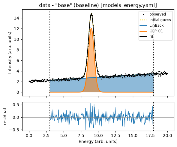
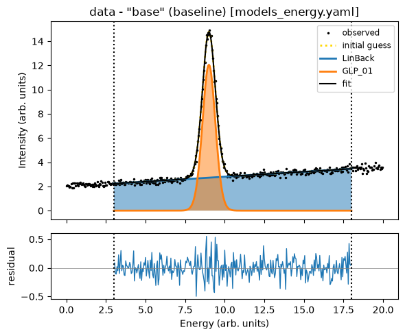
2. The Same Fit, Unweighted#
Same model, same data, same call as 12 — reusing its mc object rather than a copy of its numbers, so the noise declaration is the only difference. The fit prints the two optimizer stages; then the profiled intervals, where the GLP_01_m profile runs into its lower limit at 0 and lmfit warns Bound reached with prob(GLP_01_m=0); then the chain and its diagnostics.
# 12's baseline call, unchanged: two stages, profiled CIs, and its chain settings
file.fit_baseline(model_name="base", stages=2, try_ci=1, mc_settings=mc)
Time initialize: 2.4080276489257812e-05 s

Results global minumum fit (method=Nelder):
[[Variables]]
    LinBack_m:       0.08178424 +/- 0.00217350 (2.66%) (init = 0.0816965)
    LinBack_b:       1.98790166 +/- 0.02568673 (1.29%) (init = 1.989219)
    LinBack_xStart:  0 (fixed)
    LinBack_xStop:   20 (fixed)
    GLP_01_A:        12.0596792 +/- 0.06289779 (0.52%) (init = 12.05059)
    GLP_01_x0:       9.00139191 +/- 0.00205956 (0.02%) (init = 9.000809)
    GLP_01_F:        0.99391900 +/- 0.00523363 (0.53%) (init = 0.9940449)
    GLP_01_m:        0.23301674 +/- 0.05717134 (24.54%) (init = 0.2190757)
[[Correlations]] (unreported correlations are < 0.100)
    C(LinBack_m, LinBack_b) = -0.9164
    C(GLP_01_A, GLP_01_m)   = +0.5404
    C(GLP_01_A, GLP_01_F)   = -0.4542
    C(LinBack_b, GLP_01_F)  = -0.1721
    C(LinBack_b, GLP_01_A)  = -0.1579
    C(LinBack_b, GLP_01_m)  = -0.1427
Time fit (global minimum): 0.03209090232849121 s

Results local optimization fit (method=leastsq):
[[Variables]]
    LinBack_m:       0.08178437 +/- 0.00217330 (2.66%) (init = 0.0816965)
    LinBack_b:       1.98788813 +/- 0.02567979 (1.29%) (init = 1.989219)
    LinBack_xStart:  0 (fixed)
    LinBack_xStop:   20 (fixed)
    GLP_01_A:        12.0596777 +/- 0.06242018 (0.52%) (init = 12.05059)
    GLP_01_x0:       9.00139213 +/- 0.00205948 (0.02%) (init = 9.000809)
    GLP_01_F:        0.99391767 +/- 0.00523406 (0.53%) (init = 0.9940449)
    GLP_01_m:        0.23296556 +/- 0.05601004 (24.04%) (init = 0.2190757)
[[Correlations]] (unreported correlations are < 0.100)
    C(LinBack_m, LinBack_b) = -0.9164
    C(GLP_01_A, GLP_01_m)   = +0.5302
    C(GLP_01_A, GLP_01_F)   = -0.4533
    C(LinBack_b, GLP_01_F)  = -0.1732
    C(LinBack_b, GLP_01_A)  = -0.1562
    C(LinBack_b, GLP_01_m)  = -0.1411
Time fit (local optimization): 0.0023050308227539062 s

              99.73%    95.45%    68.27%    _BEST_    68.27%    95.45%    99.73%
 LinBack_m:  -0.00658  -0.00437  -0.00218   0.08178  +0.00218  +0.00437  +0.00658
 LinBack_b:  -0.07774  -0.05160  -0.02573   1.98789  +0.02573  +0.05158  +0.07770
 GLP_01_A :  -0.18850  -0.12556  -0.06282  12.05968  +0.06319  +0.12704  +0.19188
 GLP_01_x0:  -0.00622  -0.00414  -0.00210   9.00139  +0.00210  +0.00414  +0.00622
 GLP_01_F :  -0.01592  -0.01048  -0.00523   0.99392  +0.00526  +0.01056  +0.01596
 GLP_01_m :      -inf  -0.14336  -0.06220   0.23297  +0.05384  +0.10250  +0.14747

Progress of lmfit.emcee confidence interval determination
(based on Markov chain Monte Carlo parameter space sampling):

Results lmfit.emcee() confidence interval determination:
[[Variables]]
    LinBack_m:       0.08172091 +/- 0.00218884 (2.68%) (init = 0.08178437)
    LinBack_b:       1.98903824 +/- 0.02573887 (1.29%) (init = 1.987888)
    LinBack_xStart:  0 (fixed)
    LinBack_xStop:   20 (fixed)
    GLP_01_A:        12.0525865 +/- 0.06454390 (0.54%) (init = 12.05968)
    GLP_01_x0:       9.00126530 +/- 0.00206200 (0.02%) (init = 9.001392)
    GLP_01_F:        0.99259924 +/- 0.00579414 (0.58%) (init = 0.9939177)
    GLP_01_m:        0.22466549 +/- 0.06107674 (27.19%) (init = 0.2329656)
    __lnsigma:      -1.82181583 +/- 0.04144402 (2.27%) (init = -1.833219)
[[Correlations]] (unreported correlations are < 0.100)
    C(LinBack_m, LinBack_b) = -0.9115
    C(GLP_01_A, GLP_01_m)   = +0.5600
    C(GLP_01_A, GLP_01_F)   = -0.2922
    C(GLP_01_F, GLP_01_m)   = +0.2260
    C(LinBack_b, GLP_01_F)  = -0.1967
    C(LinBack_b, GLP_01_A)  = -0.1762
    C(LinBack_b, GLP_01_m)  = -0.1655
    C(LinBack_m, GLP_01_A)  = +0.1050
Time lmfit.emcee: 14.311461687088013 s
None
Time elapsed for baseline fit: 19.053(ss.ms)
<site-packages>/lmfit/confidence.py:356: UserWarning: Bound reached with prob(GLP_01_m=0) = 0.9873763705831702 < max(sigmas)
  warn(errmsg)
100%|██████████| 6000/6000 [00:14<00:00, 423.08it/s]
| par[v]/sigma[>] | -3.0 | -2.0 | -1.0 | best fit | +1.0 | +2.0 | +3.0 | |
|---|---|---|---|---|---|---|---|---|
| 0 | LinBack_m | 0.075178 | 0.077361 | 0.079511 | 0.081721 | 0.083890 | 0.085994 | 0.088279 |
| 1 | LinBack_b | 1.912581 | 1.938299 | 1.963712 | 1.989038 | 2.015194 | 2.041282 | 2.065875 |
| 2 | GLP_01_A | 11.864022 | 11.928736 | 11.989616 | 12.052586 | 12.118713 | 12.184618 | 12.247690 |
| 3 | GLP_01_x0 | 8.995150 | 8.997132 | 8.999236 | 9.001265 | 9.003361 | 9.005520 | 9.007591 |
| 4 | GLP_01_F | 0.969431 | 0.980158 | 0.986796 | 0.992599 | 0.998387 | 1.003918 | 1.009276 |
| 5 | GLP_01_m | 0.006094 | 0.069362 | 0.159165 | 0.224665 | 0.281329 | 0.330327 | 0.378368 |
| 6 | __lnsigma | -1.941876 | -1.902342 | -1.863560 | -1.821816 | -1.780665 | -1.739267 | -1.700619 |
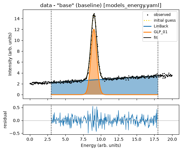
| name | value | standard error | relative error | initial value | min | max | vary |
|---|---|---|---|---|---|---|---|
| LinBack_m | 0.08178437 | 0.00217330 | (2.66%) | 0.08169650246778803 | -1.00000000 | 1.00000000 | True |
| LinBack_b | 1.98788813 | 0.02567979 | (1.29%) | 1.9892191460671924 | -5.00000000 | 5.00000000 | True |
| LinBack_xStart | 0.00000000 | 0.00000000 | 0.0 | -inf | inf | False | |
| LinBack_xStop | 20.0000000 | 0.00000000 | (0.00%) | 20.0 | -inf | inf | False |
| GLP_01_A | 12.0596777 | 0.06242018 | (0.52%) | 12.050590868232305 | 5.00000000 | 15.0000000 | True |
| GLP_01_x0 | 9.00139213 | 0.00205948 | (0.02%) | 9.000809485919255 | 5.00000000 | 15.0000000 | True |
| GLP_01_F | 0.99391767 | 0.00523406 | (0.53%) | 0.9940449226960433 | 0.75000000 | 2.50000000 | True |
| GLP_01_m | 0.23296556 | 0.05601004 | (24.04%) | 0.21907571777427792 | 0.00000000 | 1.00000000 | True |
# what ran, from the new slot: is_weighted is False and the sigma knobs are back
slot_unknown = project.results.find(file=file.name, fit_type="baseline")[-1]
print(f"resolved MC settings: {slot_unknown.fit_settings['mc']}")
print(f"chi2_red = {slot_unknown.metrics['chi2_red']}")
resolved MC settings: {'use_mc': 1, 'steps': 6000, 'nwalkers': 20, 'burn': 600, 'thin': 1, 'ntemps': 1, 'is_weighted': False, 'sigma_ini': 0.1598980933063367, 'sigma_min': 0.0015989809330633669, 'sigma_max': 15.989809330633669, 'seed': 1}
chi2_red = nan
# tier 3 under 'unknown': one extra row for the sampled noise scale
mcmc_unknown = file.get_mcmc(fit_type="baseline")
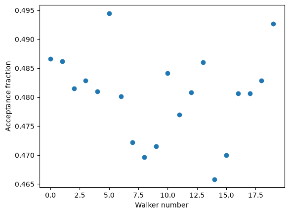
print(f"acceptance fraction: {mcmc_unknown.acceptance_fraction.mean():.2f}")
mcmc_unknown.table
acceptance fraction: 0.48
| par[v]/sigma[>] | -3.0 | -2.0 | -1.0 | best fit | +1.0 | +2.0 | +3.0 | |
|---|---|---|---|---|---|---|---|---|
| 0 | LinBack_m | 0.075178 | 0.077361 | 0.079511 | 0.081721 | 0.083890 | 0.085994 | 0.088279 |
| 1 | LinBack_b | 1.912581 | 1.938299 | 1.963712 | 1.989038 | 2.015194 | 2.041282 | 2.065875 |
| 2 | GLP_01_A | 11.864022 | 11.928736 | 11.989616 | 12.052586 | 12.118713 | 12.184618 | 12.247690 |
| 3 | GLP_01_x0 | 8.995150 | 8.997132 | 8.999236 | 9.001265 | 9.003361 | 9.005520 | 9.007591 |
| 4 | GLP_01_F | 0.969431 | 0.980158 | 0.986796 | 0.992599 | 0.998387 | 1.003918 | 1.009276 |
| 5 | GLP_01_m | 0.006094 | 0.069362 | 0.159165 | 0.224665 | 0.281329 | 0.330327 | 0.378368 |
| 6 | __lnsigma | -1.941876 | -1.902342 | -1.863560 | -1.821816 | -1.780665 | -1.739267 | -1.700619 |
__lnsigma is the noise scale emcee samples when the residual is not already in units of σ: one constant σ over the fit window, its logarithm sampled alongside the model parameters. It costs a dimension, so nwalkers derives as 2 × (free parameters + 1); that is still under the floor of 20 here, and the chain runs the same 20 walkers as 12’s. It also needs a starting point. sigma_ini defaults to the fit’s RMS residual, with the sampling bounds two decades either side of it, and §4 starts it somewhere else on purpose.
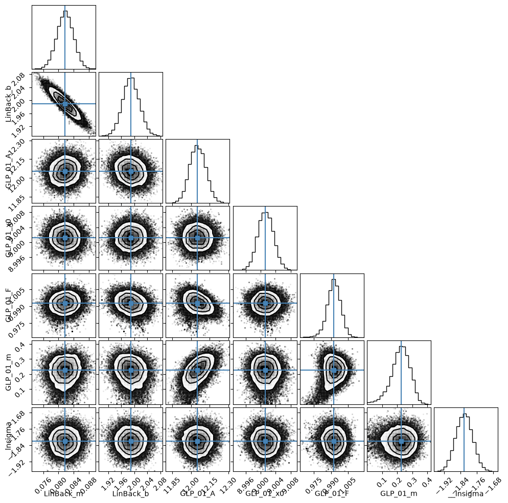
In the corner plot the fit drew, the __lnsigma row barely correlates with any model parameter — none of its correlations reach the 0.1 threshold lmfit’s fit report prints. The extra dimension is cheap, and it is not where the trouble is. The posterior above is a fair posterior for the model one constant, unknown σ; that model is the problem, on data whose σ changes from pixel to pixel.
Nothing in the output says so. chi2_red is the weighted χ² per degree of freedom, and under unknown there is no weighted χ², so the slot records nan: the gate 12 reads after every fit does not exist here. A misweighted fit and a well-weighted one print the same diagnostics.
3. The Three Tiers Next to 12’s#
Notebook 12’s baseline fit is still in the history. Pick it out by the noise it was made under, pass its handle to the same accessors, and the two sets of tiers line up parameter by parameter.
# 12's baseline slot, identified by its noise model rather than its position
slot_poisson = next(
    s
    for s in project.results.find(file=file.name, fit_type="baseline")
    if s.noise_type == "poisson"
)
# the three tiers of each fit, keyed by parameter name
pars_poisson = file.get_parameters(handle=slot_poisson.handle).set_index("name")
pars_unknown = file.get_parameters(handle=slot_unknown.handle).set_index("name")
tiers = {
    ("stderr", "poisson"): pars_poisson["stderr"],
    ("stderr", "unknown"): pars_unknown["stderr"],
    ("ci", "poisson"): one_sigma_halfwidth(
        file.get_confidence_intervals(handle=slot_poisson.handle)
    ),
    ("ci", "unknown"): one_sigma_halfwidth(
        file.get_confidence_intervals(handle=slot_unknown.handle)
    ),
    ("mcmc", "poisson"): one_sigma_halfwidth(
        file.get_mcmc(handle=slot_poisson.handle).table
    ),
    ("mcmc", "unknown"): one_sigma_halfwidth(mcmc_unknown.table),
}
# the free model parameters, in the order the fit reports them
free_pars = [n for n, row in pars_unknown.iterrows() if row["vary"] and n in truth]
# one row per parameter and tier: the two half-widths and their ratio
rows_tiers = [
    {
        "parameter": name,
        "tier": tier,
        "poisson": tiers[tier, "poisson"][name],
        "unknown": tiers[tier, "unknown"][name],
        "unknown / poisson": tiers[tier, "unknown"][name]
        / tiers[tier, "poisson"][name],
    }
    for name in free_pars
    for tier in ("stderr", "ci", "mcmc")
]
pd.DataFrame(rows_tiers).round(4)
| parameter | tier | poisson | unknown | unknown / poisson | |
|---|---|---|---|---|---|
| 0 | LinBack_m | stderr | 0.0018 | 0.0022 | 1.1874 |
| 1 | LinBack_m | ci | 0.0018 | 0.0022 | 1.1899 |
| 2 | LinBack_m | mcmc | 0.0018 | 0.0022 | 1.1843 |
| 3 | LinBack_b | stderr | 0.0206 | 0.0257 | 1.2471 |
| 4 | LinBack_b | ci | 0.0206 | 0.0257 | 1.2496 |
| 5 | LinBack_b | mcmc | 0.0205 | 0.0257 | 1.2566 |
| 6 | GLP_01_A | stderr | 0.1113 | 0.0624 | 0.5608 |
| 7 | GLP_01_A | ci | 0.1115 | 0.0630 | 0.5649 |
| 8 | GLP_01_A | mcmc | 0.1115 | 0.0645 | 0.5789 |
| 9 | GLP_01_x0 | stderr | 0.0030 | 0.0021 | 0.6867 |
| 10 | GLP_01_x0 | ci | 0.0030 | 0.0021 | 0.7010 |
| 11 | GLP_01_x0 | mcmc | 0.0030 | 0.0021 | 0.6856 |
| 12 | GLP_01_F | stderr | 0.0070 | 0.0052 | 0.7452 |
| 13 | GLP_01_F | ci | 0.0071 | 0.0052 | 0.7391 |
| 14 | GLP_01_F | mcmc | 0.0073 | 0.0058 | 0.7904 |
| 15 | GLP_01_m | stderr | 0.0706 | 0.0560 | 0.7931 |
| 16 | GLP_01_m | ci | 0.0729 | 0.0580 | 0.7955 |
| 17 | GLP_01_m | mcmc | 0.0794 | 0.0611 | 0.7689 |
# which set of error bars is the right size: the Cramér-Rao bound notebook 12
# computed from the truth model, and the pull each fit gets against the truth
rows_cal = [
    {
        "parameter": name,
        "truth": truth[name],
        "fit_unknown": pars_unknown.loc[name, "value"],
        "crb": bound[name],
        "stderr_poisson / crb": pars_poisson.loc[name, "stderr"] / bound[name],
        "stderr_unknown / crb": pars_unknown.loc[name, "stderr"] / bound[name],
        "pull_poisson": (pars_poisson.loc[name, "value"] - truth[name])
        / pars_poisson.loc[name, "stderr"],
        "pull_unknown": (pars_unknown.loc[name, "value"] - truth[name])
        / pars_unknown.loc[name, "stderr"],
    }
    for name in free_pars
]
pd.DataFrame(rows_cal).round(4)
| parameter | truth | fit_unknown | crb | stderr_poisson / crb | stderr_unknown / crb | pull_poisson | pull_unknown | |
|---|---|---|---|---|---|---|---|---|
| 0 | LinBack_m | 0.08 | 0.0818 | 0.0018 | 1.0006 | 1.1881 | 0.9269 | 0.8210 |
| 1 | LinBack_b | 2.00 | 1.9879 | 0.0206 | 0.9991 | 1.2460 | -0.5236 | -0.4716 |
| 2 | GLP_01_A | 12.00 | 12.0597 | 0.1114 | 0.9991 | 0.5603 | 0.4545 | 0.9561 |
| 3 | GLP_01_x0 | 9.00 | 9.0014 | 0.0030 | 0.9920 | 0.6812 | 0.2699 | 0.6760 |
| 4 | GLP_01_F | 1.00 | 0.9939 | 0.0077 | 0.9172 | 0.6835 | -0.8478 | -1.1621 |
| 5 | GLP_01_m | 0.25 | 0.2330 | 0.0660 | 1.0705 | 0.8490 | -0.4379 | -0.3041 |
The tiers move together. For each parameter the ratio barely changes from one tier to the next. The three are not independent estimates that happen to agree — all three are built on the single variance lmfit read off the residuals, and they inherit its error together. Agreement between tiers checks the shape of the χ² surface, not the noise model.
The direction depends on where the counts are. The two background parameters come out wider than under the declared noise, the four peak parameters narrower. One variance spread over the whole window overstates the noise on the flat background, where the counts and their Poisson scatter are small, and understates it under the peak, where the scatter is largest. The fit weights every pixel alike, and the error bars follow.
The bound settles which set is right. Under the declared noise stderr sits on the Cramér-Rao bound; under unknown all four peak parameters land below it, GLP_01_A at little more than half. A standard deviation below the bound is not something an unbiased estimator can reach, so those error bars are not standard deviations of anything. (GLP_01_F and GLP_01_m carry a wrinkle of their own, which is why even the declared-noise column is not exactly 1 for them: the bound is computed from the truth model and the covariance at the fitted point.)
The pulls do not catch any of this. Each uses its own fit’s value and error bar; the two objectives have slightly different minima. Under both declarations the pulls stay unremarkable, the largest a little over one σ. Six numbers from one realization cannot resolve a factor of two in a width. That is the uncomfortable part of the default: every check available from inside the fit looks healthy.
4. The 2D Chain, Twice#
Notebook 12 ran one short chain on the 2D fit to show how to read its convergence. Here the same short chain runs twice under unknown, differing in one input: where the sampled noise scale starts. The first takes the default, the fit’s own RMS residual. The second starts ten times too low, which is what a stale or mistyped noise estimate does.
Both chains need a scale to be checked against, and the baseline block supplies one without a model. Nothing evolves in the slices notebook 01 averaged into the ground-state spectrum, so the spread over time there is noise. Where σ varies from pixel to pixel, the root-mean-square over the fitted pixels is the summary that keeps a χ²-style check honest, since χ² averages squared residuals and their expectation is σᵢ².
# the model-free estimate: base_t_ind holds the slice range notebook 01 passed
# to define_baseline, e_lim the energy window it fits.
t_ind, e_ind = file.base_t_ind, file.e_lim
base_block = file.data[t_ind[0] : t_ind[1], e_ind[0] : e_ind[1]]
# one scalar for a signal-dependent sigma: the RMS over the fitted pixels
sigma_est = np.sqrt(base_block.var(axis=0, ddof=1).mean())
print(f"sigma_est = {sigma_est:.4f}  (per time slice, RMS over the fit window)")
sigma_est = 1.0080 (per time slice, RMS over the fit window)
# 12's short-chain settings, reused: the start of the noise scale is derived
file.fit_2d(model_name="2D", stages=2, try_ci=0, mc_settings=mc_2d)
Time initialize: 1.0967254638671875e-05 s

Results global minumum fit (method=Nelder):
[[Variables]]
    LinBack_m:                0.08178437 (fixed)
    LinBack_b:                1.987888 (fixed)
    LinBack_xStart:           0 (fixed)
    LinBack_xStop:            20 (fixed)
    GLP_01_A:                 12.05968 (fixed)
    GLP_01_x0:                9.00028517 +/- 0.00145412 (0.02%) (init = 9.001392)
    GLP_01_x0_gaussCONV_SD:   3.00424019 +/- 0.00643123 (0.21%) (init = 2.997346)
    GLP_01_x0_expFun_01_A:    5.00052143 +/- 0.00262879 (0.05%) (init = 5.000748)
    GLP_01_x0_expFun_01_tau:  49.9835767 +/- 0.04411374 (0.09%) (init = 49.99445)
    GLP_01_x0_expFun_01_t0:   0 (fixed)
    GLP_01_F:                 0.9939177 (fixed)
    GLP_01_m:                 0.2329656 (fixed)
[[Correlations]] (unreported correlations are < 0.100)
    C(GLP_01_x0, GLP_01_x0_expFun_01_tau)             = -0.6511
    C(GLP_01_x0, GLP_01_x0_expFun_01_A)               = -0.5403
    C(GLP_01_x0_gaussCONV_SD, GLP_01_x0_expFun_01_A)  = +0.4292
    C(GLP_01_x0, GLP_01_x0_gaussCONV_SD)              = -0.2636
    C(GLP_01_x0_expFun_01_A, GLP_01_x0_expFun_01_tau) = -0.1487
Time fit (global minimum): 1.102480173110962 s

Results local optimization fit (method=leastsq):
[[Variables]]
    LinBack_m:                0.08178437 (fixed)
    LinBack_b:                1.987888 (fixed)
    LinBack_xStart:           0 (fixed)
    LinBack_xStop:            20 (fixed)
    GLP_01_A:                 12.05968 (fixed)
    GLP_01_x0:                9.00027994 +/- 0.00145395 (0.02%) (init = 9.001392)
    GLP_01_x0_gaussCONV_SD:   3.00427372 +/- 0.00652788 (0.22%) (init = 2.997346)
    GLP_01_x0_expFun_01_A:    5.00053426 +/- 0.00262551 (0.05%) (init = 5.000748)
    GLP_01_x0_expFun_01_tau:  49.9836073 +/- 0.04408204 (0.09%) (init = 49.99445)
    GLP_01_x0_expFun_01_t0:   0 (fixed)
    GLP_01_F:                 0.9939177 (fixed)
    GLP_01_m:                 0.2329656 (fixed)
[[Correlations]] (unreported correlations are < 0.100)
    C(GLP_01_x0, GLP_01_x0_expFun_01_tau)             = -0.6526
    C(GLP_01_x0, GLP_01_x0_expFun_01_A)               = -0.5388
    C(GLP_01_x0_gaussCONV_SD, GLP_01_x0_expFun_01_A)  = +0.4300
    C(GLP_01_x0, GLP_01_x0_gaussCONV_SD)              = -0.2560
    C(GLP_01_x0_expFun_01_A, GLP_01_x0_expFun_01_tau) = -0.1494
Time fit (local optimization): 0.05599474906921387 s

Progress of lmfit.emcee confidence interval determination
(based on Markov chain Monte Carlo parameter space sampling):
The chain is shorter than 50 times the integrated autocorrelation time for 5 parameter(s). Use this estimate with caution and run a longer chain!
N/50 = 10;
tau: [26.68931445 30.26453636 27.3434624  24.09242298 28.62851094]

Results lmfit.emcee() confidence interval determination:
[[Variables]]
    LinBack_m:                0.08178437 (fixed)
    LinBack_b:                1.987888 (fixed)
    LinBack_xStart:           0 (fixed)
    LinBack_xStop:            20 (fixed)
    GLP_01_A:                 12.05968 (fixed)
    GLP_01_x0:                9.00004950 +/- 0.00134882 (0.01%) (init = 9.00028)
    GLP_01_x0_gaussCONV_SD:   3.00384896 +/- 0.00679514 (0.23%) (init = 3.004274)
    GLP_01_x0_expFun_01_A:    5.00087536 +/- 0.00251535 (0.05%) (init = 5.000534)
    GLP_01_x0_expFun_01_tau:  49.9884554 +/- 0.04496036 (0.09%) (init = 49.98361)
    GLP_01_x0_expFun_01_t0:   0 (fixed)
    GLP_01_F:                 0.9939177 (fixed)
    GLP_01_m:                 0.2329656 (fixed)
    __lnsigma:                0.00178023 +/- 0.00165884 (93.18%) (init = 0.001514632)
[[Correlations]] (unreported correlations are < 0.100)
    C(GLP_01_x0, GLP_01_x0_expFun_01_tau)             = -0.6524
    C(GLP_01_x0, GLP_01_x0_expFun_01_A)               = -0.4472
    C(GLP_01_x0_gaussCONV_SD, GLP_01_x0_expFun_01_A)  = +0.3852
    C(GLP_01_x0, GLP_01_x0_gaussCONV_SD)              = -0.2917
    C(GLP_01_x0_expFun_01_A, GLP_01_x0_expFun_01_tau) = -0.2536
Time lmfit.emcee: 57.32832360267639 s
None
Time elapsed for 2D model fit: 01:00.508(mm:ss.ms)
100%|██████████| 500/500 [00:57<00:00, 8.74it/s]
| par[v]/sigma[>] | -3.0 | -2.0 | -1.0 | best fit | +1.0 | +2.0 | +3.0 | |
|---|---|---|---|---|---|---|---|---|
| 0 | GLP_01_x0 | 8.995924 | 8.997185 | 8.998668 | 9.000049 | 9.001366 | 9.002742 | 9.004498 |
| 1 | GLP_01_x0_gaussCONV_SD | 2.984835 | 2.991085 | 2.997574 | 3.003849 | 3.011165 | 3.017422 | 3.023391 |
| 2 | GLP_01_x0_expFun_01_A | 4.993411 | 4.995529 | 4.998377 | 5.000875 | 5.003408 | 5.005746 | 5.008499 |
| 3 | GLP_01_x0_expFun_01_tau | 49.859329 | 49.896081 | 49.943631 | 49.988455 | 50.033577 | 50.078823 | 50.109202 |
| 4 | __lnsigma | -0.002995 | -0.001633 | 0.000185 | 0.001780 | 0.003503 | 0.005573 | 0.007289 |
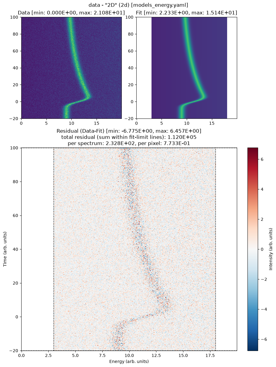
| name | value | standard error | relative error | initial value | min | max | vary |
|---|---|---|---|---|---|---|---|
| LinBack_m | 0.08178437 | 0.00000000 | (0.00%) | 0.08178437363457425 | -inf | inf | False |
| LinBack_b | 1.98788813 | 0.00000000 | (0.00%) | 1.9878881310904841 | -inf | inf | False |
| LinBack_xStart | 0.00000000 | 0.00000000 | 0.0 | -inf | inf | False | |
| LinBack_xStop | 20.0000000 | 0.00000000 | (0.00%) | 20.0 | -inf | inf | False |
| GLP_01_A | 12.0596777 | 0.00000000 | (0.00%) | 12.059677737505654 | -inf | inf | False |
| GLP_01_x0 | 9.00027994 | 0.00145395 | (0.02%) | 9.001392128660378 | 5.00000000 | 15.0000000 | True |
| GLP_01_x0_gaussCONV_SD | 3.00427372 | 0.00652788 | (0.22%) | 2.997346123480239 | 1.0000e-06 | 10.0000000 | True |
| GLP_01_x0_expFun_01_A | 5.00053426 | 0.00262551 | (0.05%) | 5.0007477105546885 | 0.00000000 | 15.0000000 | True |
| GLP_01_x0_expFun_01_tau | 49.9836073 | 0.04408204 | (0.09%) | 49.99444527268162 | 1.00000000 | 100.000000 | True |
| GLP_01_x0_expFun_01_t0 | 0.00000000 | 0.00000000 | 0.0 | -inf | inf | False | |
| GLP_01_F | 0.99391767 | 0.00000000 | (0.00%) | 0.9939176717820972 | -inf | inf | False |
| GLP_01_m | 0.23296556 | 0.00000000 | (0.00%) | 0.23296555772748267 | -inf | inf | False |
# the same chain, started ten times too low. Everything else is read off
# 12's object rather than retyped.
mc_off = MC(
    use_mc=mc_2d.use_mc,
    steps=mc_2d.steps,
    burn=mc_2d.burn,
    seed=mc_2d.seed,
    sigma_ini=sigma_est / 10,  # the one difference
)
file.fit_2d(model_name="2D", stages=2, try_ci=0, mc_settings=mc_off)
Time initialize: 1.1920928955078125e-05 s

Results global minumum fit (method=Nelder):
[[Variables]]
    LinBack_m:                0.08178437 (fixed)
    LinBack_b:                1.987888 (fixed)
    LinBack_xStart:           0 (fixed)
    LinBack_xStop:            20 (fixed)
    GLP_01_A:                 12.05968 (fixed)
    GLP_01_x0:                9.00027731 +/- 0.00145412 (0.02%) (init = 9.001392)
    GLP_01_x0_gaussCONV_SD:   3.00422926 +/- 0.00643121 (0.21%) (init = 3.004274)
    GLP_01_x0_expFun_01_A:    5.00054513 +/- 0.00262880 (0.05%) (init = 5.000534)
    GLP_01_x0_expFun_01_tau:  49.9837501 +/- 0.04411422 (0.09%) (init = 49.98361)
    GLP_01_x0_expFun_01_t0:   0 (fixed)
    GLP_01_F:                 0.9939177 (fixed)
    GLP_01_m:                 0.2329656 (fixed)
[[Correlations]] (unreported correlations are < 0.100)
    C(GLP_01_x0, GLP_01_x0_expFun_01_tau)             = -0.6511
    C(GLP_01_x0, GLP_01_x0_expFun_01_A)               = -0.5403
    C(GLP_01_x0_gaussCONV_SD, GLP_01_x0_expFun_01_A)  = +0.4292
    C(GLP_01_x0, GLP_01_x0_gaussCONV_SD)              = -0.2636
    C(GLP_01_x0_expFun_01_A, GLP_01_x0_expFun_01_tau) = -0.1487
Time fit (global minimum): 0.8524796962738037 s

Results local optimization fit (method=leastsq):
[[Variables]]
    LinBack_m:                0.08178437 (fixed)
    LinBack_b:                1.987888 (fixed)
    LinBack_xStart:           0 (fixed)
    LinBack_xStop:            20 (fixed)
    GLP_01_A:                 12.05968 (fixed)
    GLP_01_x0:                9.00027993 +/- 0.00145395 (0.02%) (init = 9.001392)
    GLP_01_x0_gaussCONV_SD:   3.00427461 +/- 0.00652784 (0.22%) (init = 3.004274)
    GLP_01_x0_expFun_01_A:    5.00053446 +/- 0.00262551 (0.05%) (init = 5.000534)
    GLP_01_x0_expFun_01_tau:  49.9836074 +/- 0.04408195 (0.09%) (init = 49.98361)
    GLP_01_x0_expFun_01_t0:   0 (fixed)
    GLP_01_F:                 0.9939177 (fixed)
    GLP_01_m:                 0.2329656 (fixed)
[[Correlations]] (unreported correlations are < 0.100)
    C(GLP_01_x0, GLP_01_x0_expFun_01_tau)             = -0.6526
    C(GLP_01_x0, GLP_01_x0_expFun_01_A)               = -0.5388
    C(GLP_01_x0_gaussCONV_SD, GLP_01_x0_expFun_01_A)  = +0.4300
    C(GLP_01_x0, GLP_01_x0_gaussCONV_SD)              = -0.2560
    C(GLP_01_x0_expFun_01_A, GLP_01_x0_expFun_01_tau) = -0.1494
Time fit (local optimization): 0.06465816497802734 s

Progress of lmfit.emcee confidence interval determination
(based on Markov chain Monte Carlo parameter space sampling):
The chain is shorter than 50 times the integrated autocorrelation time for 5 parameter(s). Use this estimate with caution and run a longer chain!
N/50 = 10;
tau: [24.43129146 41.52595945 33.09635502 22.81358544 56.81028655]

Results lmfit.emcee() confidence interval determination:
[[Variables]]
    LinBack_m:                0.08178437 (fixed)
    LinBack_b:                1.987888 (fixed)
    LinBack_xStart:           0 (fixed)
    LinBack_xStop:            20 (fixed)
    GLP_01_A:                 12.05968 (fixed)
    GLP_01_x0:                9.09003269 +/- 0.48430841 (5.33%) (init = 9.00028)
    GLP_01_x0_gaussCONV_SD:   7.54933288 +/- 2.02739182 (26.86%) (init = 3.004275)
    GLP_01_x0_expFun_01_A:    5.39761856 +/- 0.40987158 (7.59%) (init = 5.000534)
    GLP_01_x0_expFun_01_tau:  45.9533258 +/- 8.40365513 (18.29%) (init = 49.98361)
    GLP_01_x0_expFun_01_t0:   0 (fixed)
    GLP_01_F:                 0.9939177 (fixed)
    GLP_01_m:                 0.2329656 (fixed)
    __lnsigma:                0.27956441 +/- 0.22741415 (81.35%) (init = -2.294582)
[[Correlations]] (unreported correlations are < 0.100)
    C(GLP_01_x0, GLP_01_x0_expFun_01_tau)              = -0.9814
    C(GLP_01_x0_gaussCONV_SD, GLP_01_x0_expFun_01_A)   = +0.7523
    C(GLP_01_x0_gaussCONV_SD, __lnsigma)               = +0.7273
    C(GLP_01_x0_expFun_01_A, GLP_01_x0_expFun_01_tau)  = -0.7094
    C(GLP_01_x0, GLP_01_x0_expFun_01_A)                = +0.6582
    C(GLP_01_x0_expFun_01_A, __lnsigma)                = +0.4795
    C(GLP_01_x0_gaussCONV_SD, GLP_01_x0_expFun_01_tau) = -0.2520
    C(GLP_01_x0, GLP_01_x0_gaussCONV_SD)               = +0.2459
Time lmfit.emcee: 55.071189641952515 s
None
Time elapsed for 2D model fit: 57.844(ss.ms)
100%|██████████| 500/500 [00:54<00:00, 9.10it/s]
| par[v]/sigma[>] | -3.0 | -2.0 | -1.0 | best fit | +1.0 | +2.0 | +3.0 | |
|---|---|---|---|---|---|---|---|---|
| 0 | GLP_01_x0 | 8.195108 | 8.553988 | 8.756755 | 9.090033 | 9.725378 | 10.830449 | 11.040664 |
| 1 | GLP_01_x0_gaussCONV_SD | 3.081755 | 3.207771 | 5.017805 | 7.549333 | 9.073134 | 9.862551 | 9.993941 |
| 2 | GLP_01_x0_expFun_01_A | 4.902308 | 4.977460 | 5.116927 | 5.397619 | 5.936670 | 6.666983 | 7.264744 |
| 3 | GLP_01_x0_expFun_01_tau | 6.515114 | 13.147242 | 34.006572 | 45.953326 | 50.839033 | 57.986455 | 65.040791 |
| 4 | __lnsigma | -2.204396 | -2.167232 | 0.128465 | 0.279564 | 0.583293 | 0.853959 | 1.026839 |
| name | value | standard error | relative error | initial value | min | max | vary |
|---|---|---|---|---|---|---|---|
| LinBack_m | 0.08178437 | 0.00000000 | (0.00%) | 0.08178437363457425 | -inf | inf | False |
| LinBack_b | 1.98788813 | 0.00000000 | (0.00%) | 1.9878881310904841 | -inf | inf | False |
| LinBack_xStart | 0.00000000 | 0.00000000 | 0.0 | -inf | inf | False | |
| LinBack_xStop | 20.0000000 | 0.00000000 | (0.00%) | 20.0 | -inf | inf | False |
| GLP_01_A | 12.0596777 | 0.00000000 | (0.00%) | 12.059677737505654 | -inf | inf | False |
| GLP_01_x0 | 9.00027993 | 0.00145395 | (0.02%) | 9.001392128660378 | 5.00000000 | 15.0000000 | True |
| GLP_01_x0_gaussCONV_SD | 3.00427461 | 0.00652784 | (0.22%) | 3.004273719975694 | 1.0000e-06 | 10.0000000 | True |
| GLP_01_x0_expFun_01_A | 5.00053446 | 0.00262551 | (0.05%) | 5.000534261422038 | 0.00000000 | 15.0000000 | True |
| GLP_01_x0_expFun_01_tau | 49.9836074 | 0.04408195 | (0.09%) | 49.98360733603487 | 1.00000000 | 100.000000 | True |
| GLP_01_x0_expFun_01_t0 | 0.00000000 | 0.00000000 | 0.0 | -inf | inf | False | |
| GLP_01_F | 0.99391767 | 0.00000000 | (0.00%) | 0.9939176717820972 | -inf | inf | False |
| GLP_01_m | 0.23296556 | 0.00000000 | (0.00%) | 0.23296555772748267 | -inf | inf | False |
# the two chains, in history order
slots_2d = project.results.find(file=file.name, fit_type="2d")
mcmc_derived = file.get_mcmc(handle=slots_2d[-2].handle)
mcmc_off = file.get_mcmc(handle=slots_2d[-1].handle)
for label, chain, slot in (
    ("derived start", mcmc_derived, slots_2d[-2]),
    ("off-scale start", mcmc_off, slots_2d[-1]),
):
    print(
        f"{label:>16}:  sigma_ini {slot.fit_settings['mc']['sigma_ini']:.4f}"
        f"  ->  sampled sigma {np.exp(chain.lnsigma):.4f}"
        f"   acceptance {chain.acceptance_fraction.mean():.2f}"
    )
print(f"{'model-free':>16}:  sigma_est {sigma_est:.4f}")
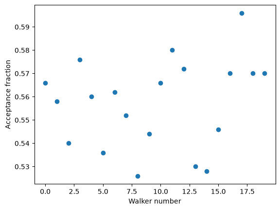
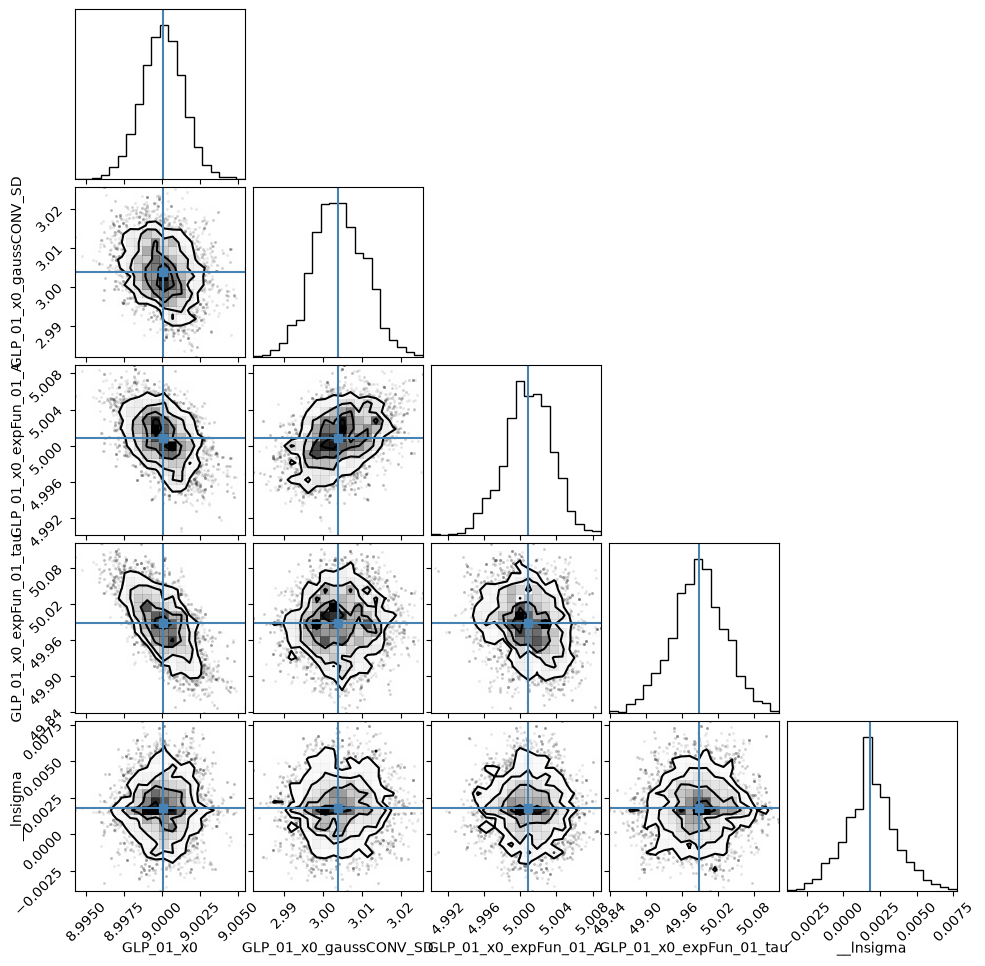
   derived start:  sigma_ini 1.0015  ->  sampled sigma 1.0018   acceptance 0.56
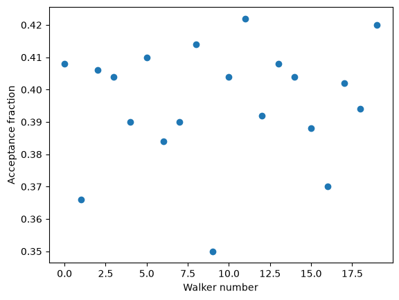
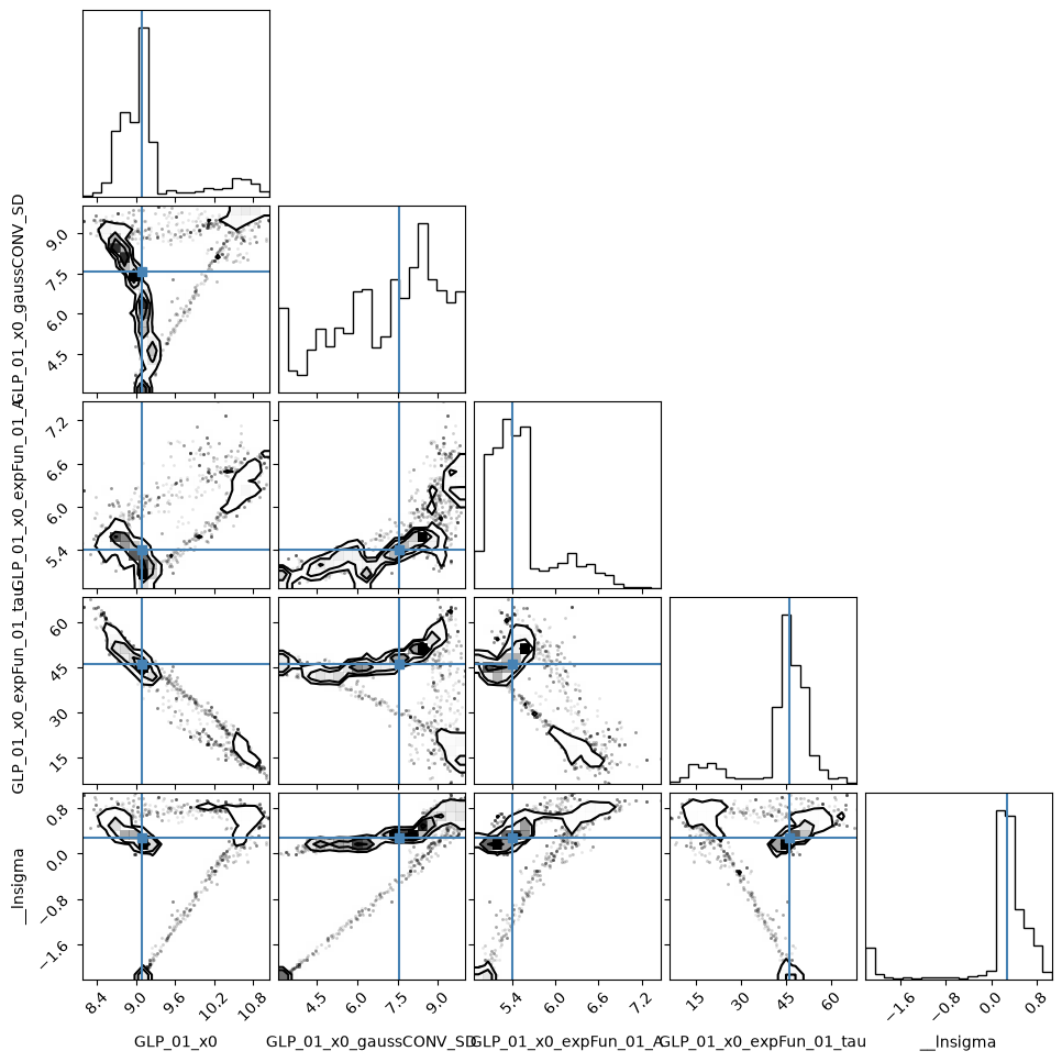
 off-scale start:  sigma_ini 0.1008  ->  sampled sigma 1.3226   acceptance 0.40
      model-free:  sigma_est 1.0080
# tier 1 is the cross-check: posterior half-widths against stderr, and against
# the widths 12's weighted chain reported for the same parameters. Both chains
# sit on the same unweighted optimizer result, so one stderr column serves both.
stderr_2d = file.get_parameters(handle=slots_2d[-2].handle).set_index("name")["stderr"]
w_derived = one_sigma_halfwidth(mcmc_derived.table)
w_off = one_sigma_halfwidth(mcmc_off.table)
w_poisson = one_sigma_halfwidth(mcmc_2d.table)
rows_2d = [
    {
        "parameter": name,
        "stderr": stderr_2d[name],
        "mcmc": w_derived[name],
        "mcmc_off": w_off[name],
        "mcmc / stderr": w_derived[name] / stderr_2d[name],
        "mcmc_off / stderr": w_off[name] / stderr_2d[name],
        "mcmc_12": w_poisson[name],
    }
    for name in w_poisson
]
pd.DataFrame(rows_2d).round(4)
| parameter | stderr | mcmc | mcmc_off | mcmc / stderr | mcmc_off / stderr | mcmc_12 | |
|---|---|---|---|---|---|---|---|
| 0 | GLP_01_x0 | 0.0015 | 0.0013 | 0.4843 | 0.9280 | 333.1006 | 0.0022 |
| 1 | GLP_01_x0_gaussCONV_SD | 0.0065 | 0.0068 | 2.0277 | 1.0411 | 310.6161 | 0.0101 |
| 2 | GLP_01_x0_expFun_01_A | 0.0026 | 0.0025 | 0.4099 | 0.9580 | 156.1110 | 0.0037 |
| 3 | GLP_01_x0_expFun_01_tau | 0.0441 | 0.0450 | 8.4162 | 1.0202 | 190.9220 | 0.0653 |
Both chains printed the same warning, “The chain is shorter than 50 times the integrated autocorrelation time”. It says emcee cannot vouch for its own τ estimate at 500 steps, not that the walkers failed to arrive. Both acceptance fractions land in or just above emcee’s healthy 0.2–0.5 band. Neither diagnostic separates the two runs.
Everything that does separate them comes from outside the chain. The chain started at the derived scale sampled a noise scale that matches the model-free sigma_est, and its posterior widths reproduce stderr parameter by parameter: a short chain that arrived. The chain started ten times too low spent its 500 steps travelling toward the right scale, never reached it, and returned widths hundreds of times stderr — no information about the parameters at all.
What the arrived chain still gets wrong is in the last column. Its widths sit well below the ones 12’s weighted chain reported, by roughly the factor §3 found for the peak parameters — every parameter free in this fit describes the peak’s position.
5. The Gaussian Fallback#
unknown is not the only fallback. Where the noise really is uniform Gaussian (an analog detector, dark-subtracted or difference data), a constant σ is the correct declaration rather than an approximation, and 10_model_comparison fits under exactly that. The σ does not have to come from the instrument either: the baseline-block estimate above is model-free.
On counting data it is the wrong declaration, but not the same kind of wrong as no declaration at all.
# one constant sigma for the whole window, from the baseline block above.
# try_ci=0 and no chain: tier 1 is enough to see what the declaration does.
file.set_noise("gaussian", sigma=sigma_est)
file.fit_baseline(model_name="base", stages=2, try_ci=0)
slot_gauss = project.results.find(file=file.name, fit_type="baseline")[-1]
print(f"chi2_red = {slot_gauss.metrics['chi2_red']:.2f}")
Time initialize: 9.298324584960938e-06 s

Results global minumum fit (method=Nelder):
[[Variables]]
    LinBack_m:       0.08178437 +/- 0.00211849 (2.59%) (init = 0.08178437)
    LinBack_b:       1.98788813 +/- 0.02503670 (1.26%) (init = 1.987888)
    LinBack_xStart:  0 (fixed)
    LinBack_xStop:   20 (fixed)
    GLP_01_A:        12.0596777 +/- 0.06131064 (0.51%) (init = 12.05968)
    GLP_01_x0:       9.00139213 +/- 0.00200743 (0.02%) (init = 9.001392)
    GLP_01_F:        0.99391767 +/- 0.00510112 (0.51%) (init = 0.9939177)
    GLP_01_m:        0.23296556 +/- 0.05574646 (23.93%) (init = 0.2329656)
[[Correlations]] (unreported correlations are < 0.100)
    C(LinBack_m, LinBack_b) = -0.9164
    C(GLP_01_A, GLP_01_m)   = +0.5405
    C(GLP_01_A, GLP_01_F)   = -0.4539
    C(LinBack_b, GLP_01_F)  = -0.1722
    C(LinBack_b, GLP_01_A)  = -0.1579
    C(LinBack_b, GLP_01_m)  = -0.1428
Time fit (global minimum): 0.03129911422729492 s

Results local optimization fit (method=leastsq):
[[Variables]]
    LinBack_m:       0.08178437 +/- 0.00211830 (2.59%) (init = 0.08178437)
    LinBack_b:       1.98788823 +/- 0.02502988 (1.26%) (init = 1.987888)
    LinBack_xStart:  0 (fixed)
    LinBack_xStop:   20 (fixed)
    GLP_01_A:        12.0596764 +/- 0.06084010 (0.50%) (init = 12.05968)
    GLP_01_x0:       9.00139214 +/- 0.00200735 (0.02%) (init = 9.001392)
    GLP_01_F:        0.99391771 +/- 0.00510153 (0.51%) (init = 0.9939177)
    GLP_01_m:        0.23296357 +/- 0.05460322 (23.44%) (init = 0.2329656)
[[Correlations]] (unreported correlations are < 0.100)
    C(LinBack_m, LinBack_b) = -0.9164
    C(GLP_01_A, GLP_01_m)   = +0.5302
    C(GLP_01_A, GLP_01_F)   = -0.4531
    C(LinBack_b, GLP_01_F)  = -0.1733
    C(LinBack_b, GLP_01_A)  = -0.1562
    C(LinBack_b, GLP_01_m)  = -0.1410
Time fit (local optimization): 0.0023589134216308594 s
Time elapsed for baseline fit: 00.299(ss.ms)
chi2_red = 1.05
| name | value | standard error | relative error | initial value | min | max | vary |
|---|---|---|---|---|---|---|---|
| LinBack_m | 0.08178437 | 0.00211830 | (2.59%) | 0.08178437363457425 | -1.00000000 | 1.00000000 | True |
| LinBack_b | 1.98788823 | 0.02502988 | (1.26%) | 1.9878881310904841 | -5.00000000 | 5.00000000 | True |
| LinBack_xStart | 0.00000000 | 0.00000000 | 0.0 | -inf | inf | False | |
| LinBack_xStop | 20.0000000 | 0.00000000 | (0.00%) | 20.0 | -inf | inf | False |
| GLP_01_A | 12.0596764 | 0.06084010 | (0.50%) | 12.059677737505654 | 5.00000000 | 15.0000000 | True |
| GLP_01_x0 | 9.00139214 | 0.00200735 | (0.02%) | 9.001392128660378 | 5.00000000 | 15.0000000 | True |
| GLP_01_F | 0.99391771 | 0.00510153 | (0.51%) | 0.9939176717820972 | 0.75000000 | 2.50000000 | True |
| GLP_01_m | 0.23296357 | 0.05460322 | (23.44%) | 0.23296555772748267 | 0.00000000 | 1.00000000 | True |
# where a constant sigma puts the error bars, against the other two declarations
stderr_gauss = file.get_parameters(handle=slot_gauss.handle).set_index("name")["stderr"]
pd.DataFrame(
    {
        "poisson": pars_poisson["stderr"],
        "unknown": pars_unknown["stderr"],
        "gaussian": stderr_gauss,
    }
).loc[free_pars].rename_axis("parameter").round(4)
| poisson | unknown | gaussian | |
|---|---|---|---|
| parameter | |||
| LinBack_m | 0.0018 | 0.0022 | 0.0021 |
| LinBack_b | 0.0206 | 0.0257 | 0.0250 |
| GLP_01_A | 0.1113 | 0.0624 | 0.0608 |
| GLP_01_x0 | 0.0030 | 0.0021 | 0.0020 |
| GLP_01_F | 0.0070 | 0.0052 | 0.0051 |
| GLP_01_m | 0.0706 | 0.0560 | 0.0546 |
# the same declaration with sigma half its estimated size
file.set_noise("gaussian", sigma=sigma_est / 2)
file.fit_baseline(model_name="base", stages=2, try_ci=0)
slot_half = project.results.find(file=file.name, fit_type="baseline")[-1]
print(f"chi2_red = {slot_half.metrics['chi2_red']:.2f}")
Time initialize: 9.5367431640625e-06 s

Results global minumum fit (method=Nelder):
[[Variables]]
    LinBack_m:       0.08178437 +/- 0.00105924 (1.30%) (init = 0.08178437)
    LinBack_b:       1.98788823 +/- 0.01251835 (0.63%) (init = 1.987888)
    LinBack_xStart:  0 (fixed)
    LinBack_xStop:   20 (fixed)
    GLP_01_A:        12.0596764 +/- 0.03065534 (0.25%) (init = 12.05968)
    GLP_01_x0:       9.00139214 +/- 0.00100372 (0.01%) (init = 9.001392)
    GLP_01_F:        0.99391771 +/- 0.00255056 (0.26%) (init = 0.9939177)
    GLP_01_m:        0.23296357 +/- 0.02787344 (11.96%) (init = 0.2329636)
[[Correlations]] (unreported correlations are < 0.100)
    C(LinBack_m, LinBack_b) = -0.9164
    C(GLP_01_A, GLP_01_m)   = +0.5405
    C(GLP_01_A, GLP_01_F)   = -0.4539
    C(LinBack_b, GLP_01_F)  = -0.1722
    C(LinBack_b, GLP_01_A)  = -0.1579
    C(LinBack_b, GLP_01_m)  = -0.1428
Time fit (global minimum): 0.03272438049316406 s

Results local optimization fit (method=leastsq):
[[Variables]]
    LinBack_m:       0.08178437 +/- 0.00105915 (1.30%) (init = 0.08178437)
    LinBack_b:       1.98788824 +/- 0.01251494 (0.63%) (init = 1.987888)
    LinBack_xStart:  0 (fixed)
    LinBack_xStop:   20 (fixed)
    GLP_01_A:        12.0596763 +/- 0.03042004 (0.25%) (init = 12.05968)
    GLP_01_x0:       9.00139214 +/- 0.00100368 (0.01%) (init = 9.001392)
    GLP_01_F:        0.99391771 +/- 0.00255077 (0.26%) (init = 0.9939177)
    GLP_01_m:        0.23296348 +/- 0.02730182 (11.72%) (init = 0.2329636)
[[Correlations]] (unreported correlations are < 0.100)
    C(LinBack_m, LinBack_b) = -0.9164
    C(GLP_01_A, GLP_01_m)   = +0.5302
    C(GLP_01_A, GLP_01_F)   = -0.4531
    C(LinBack_b, GLP_01_F)  = -0.1733
    C(LinBack_b, GLP_01_A)  = -0.1562
    C(LinBack_b, GLP_01_m)  = -0.1410
Time fit (local optimization): 0.002409219741821289 s
Time elapsed for baseline fit: 00.302(ss.ms)
chi2_red = 4.21
| name | value | standard error | relative error | initial value | min | max | vary |
|---|---|---|---|---|---|---|---|
| LinBack_m | 0.08178437 | 0.00105915 | (1.30%) | 0.08178436888759899 | -1.00000000 | 1.00000000 | True |
| LinBack_b | 1.98788824 | 0.01251494 | (0.63%) | 1.9878882347923579 | -5.00000000 | 5.00000000 | True |
| LinBack_xStart | 0.00000000 | 0.00000000 | 0.0 | -inf | inf | False | |
| LinBack_xStop | 20.0000000 | 0.00000000 | (0.00%) | 20.0 | -inf | inf | False |
| GLP_01_A | 12.0596763 | 0.03042004 | (0.25%) | 12.059676380835445 | 5.00000000 | 15.0000000 | True |
| GLP_01_x0 | 9.00139214 | 0.00100368 | (0.01%) | 9.001392139421178 | 5.00000000 | 15.0000000 | True |
| GLP_01_F | 0.99391771 | 0.00255077 | (0.26%) | 0.9939177079592996 | 0.75000000 | 2.50000000 | True |
| GLP_01_m | 0.23296348 | 0.02730182 | (11.72%) | 0.23296356748409508 | 0.00000000 | 1.00000000 | True |
The unknown and gaussian columns are within a couple of percent of each other, and that is the point: declaring one constant σ weights the fit the way unknown already did, with the number supplied instead of estimated. The Poisson column is the one sitting on the bound (§3), and neither of the others moved toward it.
What the declaration buys is the gate. chi2_red is defined again: it reads ≈ 1 for the baseline-block estimate, and about four times that for a σ declared half as large. The metric goes as 1/σ², so a factor of two in the declaration is a factor of four in the gate. A constant σ that is wrong overall cannot hide.
A constant σ that is wrong pixel by pixel can. The gate above reads 1 with the counting noise misdescribed, because the estimate matches the residuals taken as a whole. That is the failure the bound caught in §3 and the gate cannot.
Tips for a Missing Noise Model#
What unknown does
It is the default: a file carries it until
set_noiseis called. Fits under it minimize the unweighted residual and quote error bars from a covariance rescaled by the fit’s own reduced χ².All three tiers stay self-consistent under it, because all three rest on that one estimated variance. Tiers that agree tell you nothing about whether the widths are right.
There is no χ²_red gate — the metric is
nan— andcompare_modelswithholds every noise-scaled column from a group whose fits span more than one noise model.
Recognizing the damage
Misweighting is structured, not a global factor: on counting data the error bars come out too small where the signal is strongest and too large on the background.
Check from outside the fit.
sensitivity.crbneeds a model and a photon budget, no data and no fit, and anstderrbelow that bound cannot be the standard deviation of an unbiased estimator.Pulls against a known truth are a weak test on one dataset: a factor of two in the widths hides inside the normal scatter of a handful of parameters.
MCMC under unknown
The chain samples the noise scale as
__lnsigma, sonwalkersderives as 2 × (free parameters + 1) with a floor of 20, andsigma_inihas to start near the true scale. Its default, the fit’s RMS residual, is where it belongs; override it only when a structured misfit has inflated that residual.Started far off, a short chain returns confidently wrong widths while its acceptance fraction and its 50τ warning look exactly like a healthy chain’s. Compare the posterior widths against
stderr, and the sampled scale against a model-free estimate.
The fallback
set_noise('gaussian', sigma=...)with σ measured on a pre-trigger block is the right declaration when the noise is uniform, and restores the gate in every case. It does not fix signal-dependent noise: its error bars are the unweighted ones.
Next Steps#
The same data and fits with the noise declared, and all three tiers against the bound:
12_uncertainty_mcmcA known Gaussian σ where it is the right model, and the metrics it calibrates:
10_model_comparisonThe underlying fit workflow:
01_basic_fitting